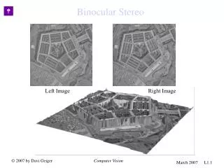
Binocular Stereo
Learn about passive and active methods for depth extraction using binocular stereo vision techniques. Explore human stereo vision examples and computer vision concepts such as Illusory Contours and Half-Occlusions. Understand the geometry of Projective Cameras and Epipolar Lines in computer vision.

Binocular Stereo
E N D
Presentation Transcript
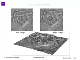
Binocular Stereo Left Image Right Image Binocular Stereo Computer Vision
Binocular Stereo • There are various different methods of extracting relative depth from images, some of the “passive ones” are based on • relative size of known objects, • texture variations, • occlusion cues, such as presence of T-Junctions, • motion information, • focusing and defocusing, • relative brightness • Moreover, there are active methods such as • Radar , which requires beams of sound waves or • Laser, uses beam of light • Stereo vision is unique because it is both passive and accurate. Computer Vision
Human Stereo: Random Dot Stereogram Julesz’s Random Dot Stereogram. The left image, a black and white image, is generated by a program that assigns black or white values at each pixel according to a random number generator. The right image is constructed from by copying the left image, but an imaginary square inside the left image is displaced a few pixels to the left and the empty space filled with black and white values chosen at random. When the stereo pair is shown, the observers can identify/match the imaginary square on both images and consequently “see” a square in front of the background. It shows that stereo matching can occur without recognition. Computer Vision
Human Stereo: Illusory Contours Stereo matching occurs in the presence of illusory. Here not only illusory figures on left and right images don’t match, but also stereo matching yields illusory figures not seen on either left or right images alone. Not even the identification/matching of illusory contour is known a priori of the stereo process. These pairs gives evidence that the human visual system does not process illusory contours/surfaces before processing binocular vision. Accordingly, binocular vision will be thereafter described as a process that does not require any recognition or contour detection a priori. Computer Vision
Left Right Left Right Human Stereo: Half Occlusions An important aspect of the stereo geometry are half-occlusions. There are regions of a left image that will have no match in the right image, and vice-versa. Unmatched regions, or half-occlusion, contain important information about the reconstruction of the scene. Even though these regions can be small they affect the overall matching scheme, because the rest of the matching must reconstruct a scene that accounts for the half-occlusion. Leonardo DaVinci had noted that the larger is the discontinuity between two surfaces the larger is the half-occlusion. Nakayama and Shimojo in 1991 have first shown stereo pair images where by adding one dot to one image, like above, therefore inducing occlusions, affected the overall matching of the stereo pair. Computer Vision
Projective Camera y Let be a point in the 3D world represented by a “world” coordinate system. Let be the center of projection of a camera where a camera reference frame is placed. The camera coordinate system has the z component perpendicular to the camera frame (where the image is produced) and the distance between the center and the camera frame is the focal length, . In this coordinate system the point is described by the vector and the projection of this point to the image (the intersection of the line with the camera frame) is given by the point , where Po=(Xo,Yo,Zo) po=(xo,yo,f) f x z f Computer Vision
y pixel coordinates O Projective Camera and Image Coordinate System where the intrinsic parameters of the camera, , represent the size of the pixels (say in millimeters) along x and y directions, the coordinate qx,qy in pixels of the image (also called the principal point) and the focal length of the camera. x We have neglected to account for the radial distortion of the lenses, which would give additional intrinsic parameters. Equation above can be described by the linear transformation Computer Vision
P=(X,Y,Z) yl yr xr Or Ol pr=(xo,yo,f) f pl=(xo,yo,f) xl f zl zr Two Projective Cameras A 3D point P, view in the cyclopean coordinate system, projected on both cameras. The same point P described by a coordinate system in the left eye is Pl and described by a coordinate system in the right eye isPr. The translation vector T brings the origin of one the left coordinate system to the origin of the right coordinate system. Computer Vision
P=(X,Y,Z) yl yr xr Or Ol pr=(xo,yo,f) f pl=(xo,yo,f) xl f zl zr Two Projective Cameras: Transformations P=(X,Y,Z) yl yr xr Or Ol pr=(xo,yo,f) f pl=(xo,yo,f) xl f zl zr The transformation of coordinate system, from left to right is described by a rotation matrix R and a translation vector T. More precisely, a point P described as Plin the left frame will be described in the right frame as Computer Vision
Two Projective Cameras Epipolar Lines P=(X,Y,Z) yl yr xr Or er el Ol pr=(xo,yo,f) pl=(xo,yo,f) xl zl zr epipolar lines Each 3D point P defines a plane . This plane intersects the two camera frames creating two corresponding epipolar lines. The line will intersect the camera planes at and , known as the epipoles. The line is common to every plane POlOl and thus the two epipoles belong to all pairs of epipolar lines (the epipoles are the “center/intersection” of all epipolar lines.) Computer Vision
Estimating Epipolar Lines and Epipoles The two vectors, , span a 2 dimensional space. Their cross product , , is perpendicular to this 2 dimensional space. Therefore where F is known as the fundamental matrix and needs to be estimated Computer Vision
Computing F (fundamental matrix) • “Eight point algorithm”: • Given two images, we need to identify eight points or more on both images, i.e., we provide n 8 points with their correspondence. The points have to be non-degenerate. • Then we have n linear and homogeneous equations • with 9 unknowns, the components of F. We need to estimate F only up to some scale factors, so there are only 8 unknowns to be computed from the n 8 linear and homogeneous equations. • If n=8 there is a unique solution (with non-degenerate points), and if n > 8 the solution is overdetermined and we can use the SVD decomposition to find the best fit solution. Computer Vision
Stereo Correspondence: Ambiguities Each potential match is represented by a square. The black ones represent the most likely scene to “explain” the images, but other combinations could have given rise to the same images (e.g., red) What makes the set of black squares preferred/unique is that they have similar disparity values, the ordering constraint is satisfied and there is a unique match for each point. Any other set that could have given rise to the two images would have disparity values varying more, and either the ordering constraint violated or the uniqueness violated. The disparity values are inversely proportional to the depth values Computer Vision
Right FE D C A E F A B D C boundary Surface orientation discontinuity depth discontinuity no match A B C D F Left no match Boundary F A D C C D B E A F Stereo Correspondence: Matching Space In the matching space, a point (or a node) represents a match of a pixel in the left image with a pixel in the right image Left Right Note 1: Depth discontinuities and very tilted surfaces can/will yield the same images ( with half occluded pixels) Note 2: Due to pixel discretization, points A and C in the right frame are neighbors. Computer Vision
For manipulating with integer coordinate values, one can also use the following representation Restricted to integer values. Thus, for l,r=0,…,N-1 we have x=0,…2N-2 and w=-N+1, .., 0, …, N-1 Note: Not every pair (x,w) have a correspondence to (l,r), when only integer coordinates are considered. For “x+w even” we have integer values for pixels r and l and for “x+w odd” we have supixel locations. Thus, the cyclopean coordinate system for integer values of (x,w) includes a subpixel image resolution x=8 Cyclopean Eye The cyclopean eye “sees” the world in 3D where x represents the coordinate system of this eye and w is the disparity axis Right Epipolar Line x r+1 r=5 r-1 w w=2 l-1 l=3 l+1 Computer Vision
x=8 x=8 Uniqueness-Opaque Given that the l=3 and r=5 are matched (blue square), then the red squares represent violations of the uniqeness-opaqueness constraint while the yellowsquares represent unique matches, in the cyclopean coordinate system but multiple matches in the left or right eyes coordinate system. x Right Epipolar Line YES, multiple match for the left eye YES, multiple match for the right eye r+1 r=5 r-1 w NO: Uniqueness NO: Uniqueness w=2 l-1 l=3 l+1 Left Epipolar Line The Uniqueness-Opaque Constraint There should be only one disparity value, one depth value, associated to each cyclopean coordinate x (see figure). The assumption is that objects are opaque and so a 3D point P, seen by the cyclopean coordinate xand disparity value w will cause all other disparity values not to be allowed. Closer points than P , along the same x coordinate, must be transparent air and further away points will not be seen since P is already been seen (opaqueness). However, multiple matches for left eye points or right eye points are allowed. This is indeed required to model tilt surfaces and occlusion surfaces as we will later discuss. This constraint is a physical motivated one and is easily understood in the cyclopean coordinate system. Computer Vision
YES YES x=8 x=8 x=8 Surface Constraints I Smoothness : In nature most surfaces are smooth in depth compared to their distance to the observer, but depth discontinuities also occur. Smoothness x Right Epipolar Line Given that the l=3 and r=5 are matched (blue square), then the red squares represent violations of the ordering constraint while the yellowsquares represent smooth matches. YES r+1 r=5 r-1 w YES w=2 l-1 l=3 l+1 Left Epipolar Line Computer Vision
x=8 Surface Constraints: Discontinuities and Occlusions x Right Epipolar Line r+1 r=5 r-1 w x=8 w Ordering Violation x w=2 l Left Epipolar Line r l-1 l=3 l+1 Discontinuities: Note that in these cases, some pixels will not be matched to any pixel, e.g., “l+1”, and other pixels will have multiple matches, e.g., “r-1”. In fact, the number of pixels unmatched in the left image is the same as the number of multiple matches in the right image. Computer Vision
Neighborhood (with no subpixel accuracy) w w x x l l r r r r x x ? ? w’=w+2 X w’=w+2 r=6 r=5 r=4 r=3 r=6 r=5 r=4 r=3 x x w’=w-2 w’=w-2 X x’=x-2-|w’-w| x’=x-2-|w’-w| w=4 w=4 l l Neighborhood structure for a node (e,xw) consisting of flat, tilt, or occluded surfaces. Note that when an occlusion/discontinuity occurs, the contrast matches on the front surface. Jumps “at the right eye” are from back to front, while jumps “at the left eye” are from front to the back. l=1 l=2l=3 l=1 l=2l=3
x Right Epipolar Line Smoothness (+Ordering) D=3 r+1 r=5 r-1 w x=8 Starting x w=2 l-1 l=3 l+1 w=-3 Limit Disparity • The search is within a range of • disparity : 2D+1 , i.e., • The rational is: • Less computations • Larger disparity matches imply larger errors in 3D estimation. • Humans only fuse stereo images within a limit. It is called the Panum’s limit. We may start the computations at x=D to avoid limiting the range of w values. In this case, we also limit the computations to up to x=2N-2-D Computer Vision
Bayesian Formulation The probability of a surface w(x,e) to account for the left and right image can be described by the Bayes formula as where e index the epipolar lines. Let us develop formulas for both probability terms on the numerator. The denominator can be computed as the normalization constant to make the probability sum to 1. Computer Vision
left right left right The Image Formation I (special case) P(e,x,w) Є [0,1], for x+w even, represents how similar the images are between pixels (e,l) in the left image and (e,r) in the right image, given that they match. We use “left” and “right” windows to account for occlusions. Computer Vision
The Image Formation I (intensity) Note that when x+w is odd, the coordinates l and r are half integers and so an interpolation/average value for the intensity values need to be computed. For half integer values of l and r we use the formulas where is the floor value of x. We expand the previous formula to include matching of windows that have other orientations than just q =0 and we expand the formula to any integer value ofx+w. Computer Vision
The Image Formation II (Occlusions) Occlusions are regions where no feature match occur. In order to consider them we introduce an “occlusion field” O(e,x) which is 1 if an occlusion occurs at column (e,x) and zero otherwise. Thus, the likelihood of left and right images given the feature match must take into account if an occlusion occurs. We modify the data probability to include occlusions. where O is an occlusion binary variable The cost l is introduced as a prior to encourage matches, otherwise it is better to occlude everything. Computer Vision
The Image Formation III (Occluded Surfaces) x and where X X and r=6 r=5 r=4 r=3 x=9 X X X Example of a jump/occlusion, w=2 and w’=-1. Three x coordinates will have O(e,x)=1 O(e,x)=1 w=2 l=1 l=2l=3 Computer Vision
The Image Formation IV (Tilted Surfaces) x and where X X and r=6 r=5 r=4 r=3 x=9 X X X Example of a jump/occlusion, w=2 and w’=-1. Three x coordinates will have O(e,x)=1 O(e,x)=1 w=2 l=1 l=2l=3 Computer Vision Computer Vision March 2010 L1.26
Posterior Model Neighborhood structure for a node (e,xw) consisting of flat, tilt, or occluded surfaces x r=6 r=5 r=4 r=3 If there is a match at (e,xw) then either it is a flat/tilt surface or it is an occluded surface X X x=9 X w=2 l=1 l=2l=3 Computer Vision
Posterior Model (with no subpixel accuracy) Neighborhood structure for a node (e,xw) consisting of flat, tilt, or occluded surfaces x x w=D r=6 r=5 r=4 r=3 r=6 r=5 r=4 r=3 ? ? w’=w+2 X x X w=-D w=4 w=2 w’=w-2 x’=x-2-|w’-w| l=1 l=2l=3 l=1 l=2l=3 Computer Vision Computer Vision March 2008 L1.28
x Flat right left r=5 r=4 r=3 X right left right left X w=2 l=1 l=2l=3 Tilted x=8 right left Need for prior model: Flat or (Double) Tilted ? w a.Flat Plane b.Doubled Tilted The data and the probabilities for (a) and (b) are the same. Since we are not considering curvature preferences, the preference for flat surfaces must be built as a prior model of surfaces. x r=5 r=4 r=3 r=2 X x=8 X X b.Tilted X a.Flat Plane The images and the probabilities for (a) and (b) are the same. w=2 l=1 l=2l=3 Computer Vision
Dynamic Programming (pixel-pixel matching only) States (2D+1) F[x,w+D]= C[x, w+D] + minx’=-D-1,..,D+1{F[x’,w(x’)+D]+F[x,x’,w,w’]} w=D w w=-D Fx[x’,w(x’)+D] F[x, w+D, i+1] ? ? ? 1 2 3 x’ … x-1 x ... 2N-2 Computer Vision Computer Vision March 2008 L1.30