Accurate Multi-View Reconstruction Using Robust Binocular Stereo and Surface Meshing
320 likes | 581 Vues
Accurate Multi-View Reconstruction Using Robust Binocular Stereo and Surface Meshing. Derek Bradley Tamy Boubekeur * Wolfgang Heidrich University of British Columbia, TU Berlin* Advisor : P rofessor HueiYung Lin Reporter : JhengYou Lin. Multi-View Stereo.

Accurate Multi-View Reconstruction Using Robust Binocular Stereo and Surface Meshing
E N D
Presentation Transcript
Accurate Multi-View Reconstruction Using Robust Binocular Stereo and Surface Meshing Derek Bradley TamyBoubekeur* Wolfgang Heidrich University of British Columbia, TU Berlin* Advisor:ProfessorHueiYung Lin Reporter:JhengYou Lin
Multi-View Stereo • We can classify MVS algorithm as following: [33] • 3D volumetric [Hornung et al, CVPR’06] • Surface evolution [Zaharescu et al, ACCV’07] • Compute and merge depth maps [Goesele et al, CVPR’06] • Grow regions or surfaces starting from seed points [Furukawa et al, CVPR’07] 3D volumetric Surface evolution Furukawa et al Goeseleet al.
Multi-View Stereo • We can classify MVS algorithm as following: [33] • 3D volumetric [Hornung et al, CVPR’06] • Surface evolution [Zaharescu et al, ACCV’07] • Compute and merge depth maps [Goesele et al, CVPR’06] • Grow regions or surfaces starting from seed points [Furukawa et al, CVPR’07] 3D volumetric Surface evolution Furukawa et al Goeseleet al.
Multi-View Stereo • Compute and merge depth maps [Goesele et al, CVPR’06] • Choose only the points that correlate well in multiple views • Reconstruction only the portion of the scene that can be matched with high confidence 3D volumetric Surface evolution Furukawa et al Goeseleet al.
Algorithm Overview • Input • Two steps
Algorithm Overview • Input : calibrated images • Two steps
Algorithm Overview • Input : calibrated images • Two steps • Binocular stereo
Algorithm Overview • Input : calibrated images • Two steps • Binocular stereo • Surface reconstruction • Down sampling、Cleaning、Meshing
They focus on accuracy and efficiency • (accuracy) produces the most accurate results for sparse number viewpoints (Middlebury datasets) • (efficiency) the most efficient method among non-GPU algorithms
Outline • Stereo Matching • Surface Reconstruction • Experimental results
Stereo Matching Rectify A compact algorithm for rectification of stereo pairs [Fusiello et al, 2000]
Stereo Matching Rectify Scaled window matching Without paying too much attention to the reliability of the stereo matches, increase stereo matches by employing a scaled window matching approach.
Stereo Matching Rectify Scaled window matching Subpixel Optimization For each pixel, perform correlation at a number of linearly interpolated positions between previous and next pixel in the scan line. Achieve subpixel precision of 1/n pixels. (n is a user defined variable)
Stereo Matching Rectify Scaled window matching Subpixel Optimization To decrease outliers Constraints Visual Hull Disparity ordering constraint [Baker et al, 1981]
Stereo Matching Rectify Scaled window matching Subpixel Optimization Constraints Filtering median-rejection filter (disparity value is rejected if sufficiently different from the median of its local neighborhood) trilateral filter (standard bilateral filter weighted by NCC value) → remove high-frequency noise
Scaled Window Matching • Primary and reference view can distort the matching window Ogale et al, IJCV 2007
Scaled Window Matching Ogale et al, IJCV 2007 Vertical scale is identical in both view. Horizontal scale depends on the 3D surface orientation.
Scaled Window Matching Vertical scale is identical in both view. Horizontal scale depends on the 3D surface orientation.
Scaled Window Matching Vertical scale is identical in both view. Horizontal scale depends on the 3D surface orientation.
Scaled Window Matching We can find best match at largest NCC value. Experimentally found that scale factors of 1/√2, 1, √2 yield excellent results. Vertical scale is identical in both view. Horizontal scale depends on the 3D surface orientation.
Surface Reconstruction Now we have a single point cloud. Generate a mesh M from the point-normal sampling by downsampling, cleaning and meshing.
Surface Reconstruction - Downsampling • Oversampling in smooth regions, apply "hierarchical vertex clustering" (recursive, no need connectivity) • Compute a bounding box B • Instantiate a hierarchical space partitioning structure H (Volume-Surface Tree [Boubekeur et al, 2006]) • Partition recursively in H until each subset reach a given error metric • Replace each subset by a single representative sample(center and normal)
Surface Reconstruction - Cleaning • Two kinds of noise • outliers (iterative_3times classification, compute the Plane Fit Criterion[42]) • small scale high frequency noise (point-normal filtering [Amenta and kil, SIGGRAPH’04]) • basically a simplification of the Moving Least Square projection[1] using the per-sample normal estimate.
Surface Reconstruction - Meshing • Use a fast interpolating meshing approach based on the Delaunay triangulation • but too slow, it can only performed efficiently with small and low dimensional point sets.
Surface Reconstruction - Meshing • Build on [8]&[6] and design an algorithm that solves the problem using following principles: • locality (split PF into clusters using a density-driven octree) • Delaunay triangulation is performed independently. • dimension reduction (project the samples in a leaf cluster onto a least-square plane) • Delaunay triangulation in 2D space defined by this plane.
Surface Reconstruction - Meshing • Establish a single connected mesh. • Volumetrically inflate each cluster by adding points from neighborhood octree cells. • Remove following classification of the triangles: • Outside • Redundant (more than one instance) • Dualpair • Valid • Remove overlapping triangles
Surface Reconstruction - Performance • Finding neighborhood in using KD-Trees • complexity: (only taking no more than few seconds)
Dino – sparse 16 images 186254 triangles Temple – 47 images Red - √2, Blue – 1/√2 869803 triangles Sleeve – 14 images (canon DLSR) 2048x1364 290171 triangles
Results for the Middlebury datasets Accuracy(Acc)、Completeness(Cmp)、Processing time(Time)