Chapter 4 Stochastic Modeling and Stochastic Timing
Chapter 4 Stochastic Modeling and Stochastic Timing. UCLA EE201C Professor Lei He. Outline. Process Variation Trends Modeling Statistic Static Timing Analysis (SSTA) Monte Carlo simulation Path-based and block-based SSTA. As Good as Models Tell ….

Chapter 4 Stochastic Modeling and Stochastic Timing
E N D
Presentation Transcript
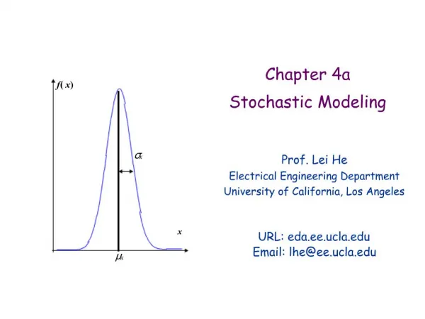
Chapter 4Stochastic Modeling and Stochastic Timing UCLA EE201C Professor Lei He
Outline • Process Variation • Trends • Modeling • Statistic Static Timing Analysis (SSTA) • Monte Carlo simulation • Path-based and block-based SSTA
As Good as Models Tell… • STA (static timing analysis) assumed: • Delays are deterministic values • Everything works at the extreme case (corner case) • Useful timing information is obtained • However, anything is as good as models tell • Is delay really deterministic? • Do all gates work at their extreme case at the same time? • Is the predicated info correlated to the measurement? • …
Factors Affecting Device Delay • Manufacturing factors • Channel length (gate length) • Channel width • Thickness of dioxide (tox) • Threshold (Vth) • … • Operation factors • Power supply fluctuation • Temperature • Coupling • … • Material physics: device fatigue • Electron migration • hot electron effects • …
Lithography Manufacturing Process • As technology scales, all kinds of sources of variations • Critical dimension (CD) control for minimum feature size • Doping density • Masking
Process Variation Trend • Keep increasing as technology scales down [Nassif 01] • Absolute process variations do not scale well • Relative process variations keep increasing
Variation Impact on Delay [Visweswariah 04] • Extreme case: guard band [-40%, 55%] • In reality, even higher as more sources of variation • Can be both pessimistic and optimistic
Variation-aware Delay Modeling • Delay can be modeled as a random variable (R.V.) • R.V. follows certain probability distribution • Some typical distributions • Normal distribution • Uniform distribution
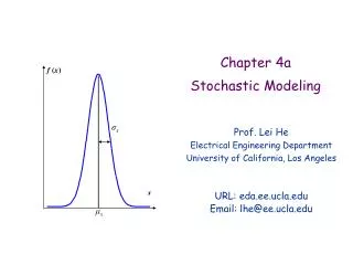
F (x) 1 f (x) dx 0 x x Review of Probability • R.V. X can take value from its domain randomly • Domain can be continuous/discrete, finite/infinite • PDF vs. CDF
f (x) σx x μx Review of Probability • Mean and Variance • Normal Distribution
Multivariate Distribution • Similar definition can be extended for multivariate cases • Joint PDF (JPDF), Covariance • Becomes much more complicated • Correlation MATTERS!!
Types of Process Variation • Inter-die vs. intra-die variations • Die to die / wafer to wafer / lot to lot • Within a single die • Random vs. systematic • CMP and OPC related • Doping density, lens aberration • Many more “confusing” terms … • OCV/ACLV • CMP • Partly due to the fact that this area is fairly new and ever changing
Variation-aware Delay Modeling • How to characterize delay variations? • SPICE simulation • Measurement • Example for a 2-stage buffer • Assume only channel length is R.V. for 65nm technology • Uniform distribution with domain ~ 10% of its nominal value • Random sample channel length from 0.9~1.1, and measure the delays through SPICE • Plot delay PDF
Variation-aware Timing Analysis • How this would affect our STA? • Min-Max approach would be too risky • Corner-based STA is too expensive • 2^n corners • To be accurate, analyze timing statistically • But how? • Every label (delays) in the DAG is modeled as a R.V. with certain distribution • Should use multivariate R.V. analysis • Correlation is KEY!
Correlation Types • Correlation interpretation: • Gates, wires, and paths become slower or faster simultaneously • Due to the common sources of underlying variations • Global variation • Inter-chip variations • Structural correlation • Path re-convergence • Spatial correlation • Devices close-by have higher correlation than that far-apart
Statistical Static Timing Analysis: SSTA • Fairly new (hot) topic • Many debates • Many new ideas • Not quite consistency across different ref. • Unfortunately/Fortunately, live with it… • In this lecture, cover some typical ones • Monte Carlo simulation (Golden case) • One path-based approach • One block-based approach • More for your own entertainment
Monte Carlo Simulation • Definition: • A technique involving the use of random numbers solving physical or mathematical problems • Characteristics • Physical process is simulated without explicitly knowing equations that describe the system output • Only requirement is that the physical system be described by PDF
Monte Carlo for SSTA • Randomly sample each R.V. in accordance with its respective PDF • Instantiate a specific DAG • Solving STA using the technique we discussed before • This is called one Monte Carlo run • Run it many times until certain data statistics converge • Stopping condition can be fairly sophisticated • Finally, extract statistics from Monte Carlo runs • PDF of RAT/AT/Slack • Yield curve • …
Monte Carlo Simulation • Pros • Conceptually easy • Implementation not that difficult • Make use of previous STA algorithm • Accurate, used as golden case (benchmarking) • Cons • Computationally expensive • No many diagnostic information if something is wrong • No incremental computation possible • Efficient solution • Analytical Statistical static timing analysis (SSTA)
SSTA Algorithms • Objective • Find probability distribution of circuit delay • Path Based SSTA • Statistically calculate path delay distributions • Find statistical maximum of these path delays • Identify potential critical paths • Block Based SSTA • Traverse DAG to calculate the delay distribution for each node • Widely used due to the incremental computation capability
Path-based SSTA [Orshansky DAC-02] • Key operations • Summation • Path delay = sum(node delay) • Maximum • Critical path delay = max(path delay) • Delay model • First order approximation • Obtained from SPICE simulation
Path-based SSTA: Key Operations • Gate delay variance and covariance • Path delay variance and covariance
Path-based SSTA: Approximation • Maximum operation is approximated • Closed form is not known yet • Lower and upper bound for path delay mean • Let D={D1...Dn } be an arbitrary path delay distribution with correlation • Let X={X1...Xn } identical to D but WITHOUT correlation • Can prove an upper bound for mean(D): • Mean(D) < Mean(X) • Similarly an lower bound can be established
Path-based SSTA: Approximation • Lower and upper bound for path delay variance • Result from theory of Gaussian process: Borell Inequality • Variance of max{D1…Dn} around its mean is smaller than variance of a single Di with largest variance
Path-based SSTA: Experiment Results • Timing approximation is tighter • Variation is smaller • Mean clock frequency is smaller
1.0 1.0 P3 Cumulative Probability P2 P1 A A3 A2 A1 Block-based SSTA: [Devgan ICCAD03] • AT and gate delays are modeled as R.V. • AT as CDFs • Gate Delays as PDFs • For easy computation • Delay distributions can take any form • Model CDFs as Piece-Wise Linear functions • Model PDFs as constant step functions
AT1 AT2 D1 1 2 ( : convolution, Assuming independence for now) AT2 = AT1 D1 PDF CDF Block-based SSTA: Key Operations • Addition AT2 = AT1+D1
s1 0.5s1u1(t1+t2-t)2 t1 t1+t2 u1 t2 Block-based SSTA: Key Operations • Closed form for addition =
s1 s1s2(t-t1)(t-t2) t1 x t3=max(t1,t2) s2 t2 Block-based SSTA: Key Operations • Maximum C = max (A, B) • CDF of C = CDF of A x CDF of B • Assume independence for now • Closed form computation via PWL =
AT1 AT2 D1 PI D6 AT5 AT4 D3 D4 D8 D9 PO D2 PI AT6 AT3 D7 Block-based SSTA: Correlation • Correlation due to path reconvergence • AT5 and AT6 are correlated due to shared AT4 • Exact handling this correlation would cause exponential complexity • Utilize the structure of the circuits
1 3 2 4 Block-based SSTA: Correlation • This formula works well for this simple case • How does this work for general cases? A4 = max(A2+D24, A3+D34) A2 and A3 are related A2 = A1 + D12andA3 = A1 + D13 A4=max(A1+D12+D24, A1+ D13+D34)=A1+max(D12+D24, D13+D34)
G2 B G1 G4 A 1 D 2 3 z 4 G3 C Block-based SSTA: General Cases • General situation • An input of a gate can depend on many preceding timing points • There may be shared paths in the input cone
Block-based SSTA: Heuristic Algorithm • Create a dependency list • Keep track of the reconvergence fanout nodes a particular node depends on • Basically a list of pointers • Compute the dominant common node • For each pair wise max • Determine that by statistical dominance and logic level • Take out the common part contributed by the dominant node • Perform max of the two CDFs • An example follows
G2 B G1 G4 1 A A B G4 D 2 z 1 3 A B C D 4 2 G3 z C A 3 C 4 C Block-based SSTA: Example Dependency list for G4: Create the dependency list
B G4 Dependency list for G4: 1 B D 2 A B z G4 C 3 1 4 A B C D 2 z C A C 3 4 C Block-based SSTA: Example Dominant common node
G4 B 1 D 2 B z 3 C 4 C Block-based SSTA: Example Compute the pair wise max ATD = max(A1+D1z, A2+ D2z, A3+D3z, A4 + D4z) ATx = AB + max(A1-AB +D1z, A2-AB+ D2z) ATy = Ac + max(A3-Ac +D3z, A4-Ac+ D4z) ATD = max (ATx, ATy)
Block-based SSTA: Experiments • Runtime comparison • SSTA w/ correlation and w/o correlation
Block-based SSTA: Experiments • Timing distribution • SSTA w/ correlation and w/o correlation and Monte Carlo Simulation
Summary • Timing analysis is a key part of the design process • Static timing analysis (STA) • Sign off tools for tape out • Statistical static timing analysis (SSTA) • Arises due to process variation when technology continues to scale • More to be done for SSTA • Correlations matter • Interconnect variability • Slew propagation • Gate delay models • How to guide for optimal design?