Understanding Stochastic Processes in Problem Solving
Learn about stochastic processes, random events evolving over time, essential for modeling outcomes. Explore binomial, Poisson, and random walk processes for predictive analysis and simulations. Understand how to estimate parameters from data.


Understanding Stochastic Processes in Problem Solving
E N D
Presentation Transcript
Stochastic Processes Eberhard O. Voit Integrative Core Problem Solving with Models November 2011
Agenda Definitions and Introductory Example Binomial (Bernoulli) Process Poisson Process Random Walk Random Walk as Markov Chain Mean time Diffusion Random Number Generation In some respect, these are the ultimate stochastic processes. Others are Markov, normal, queuing, and branching processes
“Stochastic” stoco: Aim, goal, target; guess, solution to a puzzle stocastiko: Able to hit the target, smart stocastik: Fortuneteller K.-G. Hagstroem: Skandinavisk Aktuarientidskrift 23, 54-57, 1940 Uses: English, Latin, Greek, French, German, Dutch, Swedish, Italian
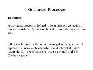
Stochastic Process Phenomenon changing over time and containing random component(s) A mathematical representation of this phenomenon ~ Probabilistic model of a dynamic process Example: Draw cards from a deck repeatedly (with or without replacement) T = {discrete time points}; t T At each t an observation is made on the random variable X(t) (e.g., X(5) = Ace) Then, {X(t): tT} is a random process or stochastic process (SP) Process may be multivariate; T is called the index set.
Stochastic Process Is anything truly stochastic? Does stochasticity depend on the observer or degree of knowledge? Examples: Random number generator The unfortunate flower pot accident
Stochastic Process Aims: Simulation of scenarios Best, worst, most likely outcomes; outcomes within certain ranges Make statements about general, average, or collective behavior Mean and variance, e.g., with respect to time In many cases, these statements refer to the statistical distribution of collective outcomes and its properties (mean, variance, moments, …) or to other distributions, which the target distribution approaches for large numbers of “trials” Recall Central Limit Theorem
Stochastic Process More Aims: Make predictions (in the face of randomness), based on distributions Estimate functional form of SP Estimate key parameters (separate signal from noise) Note: Seamless transition to time series analysis (e.g., weather forecasting) X(t) time t
Old Example: Population Growth by Cell Doubling Pt+t= 2 Pt P(t+t ) +t= 2 Pt+t = 2 2 Pt = 22Pt Randomize: Replace “2” with a random number? Make t random? Voit and Dick (1983): At division, cells are assigned a cycle duration (probabilistic) No cell death Things get out of hand quickly! Equivalent? Voit, E.O. and G. Dick: Mathem. Biosci.66, 229-246 and 247-262, 1983
Example: PopulationGrowth by Cell Doubling Voit and Dick (1983): Example: Cycle durations 5, 6, or 8 Things get out of hand quickly! Linear algebra comes to the rescue!
Example: PopulationGrowth by Cell Doubling Compute short-term and long-term population sizes: Ultimately exponential Compute age distributions over time: Ultimately stable
Other Old Examples: Dynamics of Red Blood Cells Original Equations: Rn = (1 – f)Rn-1 + Mn-1 Mn = g fRn-1 Could make f and g probabilistic
Leslie Matrix for Growth of Age-Structured Populations Markov (Chain) Models
Binomial (Bernoulli) Process Bernoullis: Swiss-Dutch family of mathematicians (over three centuries) Stochastic processes: Daniel Bernoulli (1700 – 1782) Sequence of “trials” leading to “success” or “failure” Flipping coin; checking for faulty items; mutations within DNA sequence Trials independent of each other; no learning Number of trials: n Number of successes: k Success probability per trial: p Probability of having exactly k successes:
Bernoulli Process Examples: Suppose: Mutation rate per DNA base is 0.0035 What is probability of finding exactly one mutation in a stretch of 10 bases? 0.0339 What is probability of finding exactly two mutations in a stretch of 10 bases? 0.000537
Bernoulli Process Examples: What is probability of not finding a single mutation in a stretch of 10 bases? 0.9655 What is probability of finding more than two mutations in a stretch of 10 bases? P(k > 2) = 1 - 0.9655 - 0.0339 - 0.000537 0.00002 (2 in 100,000)
Bernoulli Process Increase length of DNA; expect more mutations. E.g., n = 1,000 For exactly one mutation: 1000! is a real problem! But: 1000! = 1 2 3 … 1000; 999! = 1 2 3 … 999; 1! = 1 Thus: 1000! / 999! = 1000 Does not help much with a few hundred mutations!
Bernoulli Process Circumvent problems: 1. Sterling’s formula: (James Sterling: 1692-1770; Scot) n = 15: 27.8993 0.9189 41.9748 15 27.8937 2. Use Poisson process instead of Bernoulli process
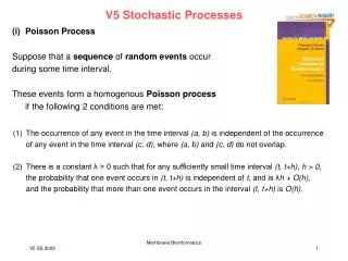
Poisson Process Siméon Denis Poisson (1781 – 1840) Poisson distribution first published in 1837: Recherches sur la probabilité des jugements en matière criminelle et en matière civile (“Research on the Probability of Judgments in Criminal and Civil Matters”). Classical examples: 1. Decay of a radioactive sample: decay is believed to be random; once a particle has decayed, it does not decay again. 2. Raindrops on a tiled sidewalk 3. Mutations within DNA sequence 4. Events in continuous spaces (number of rust spots on a metal rod)
Poisson Process If the expected number of occurrences in a given interval is l, then the probability that there are exactly k occurrences (k = 0, 1, 2, ...) is equal to Example from before: Suppose: Mutation rate per DNA base is 0.0035 What is probability of finding exactly one mutation in a stretch of 10 bases? Bernoulli: P = 0.0339 For large number of trials, and / or small rates, Bernoulli is well approximated by Poisson: Poisson: “rate” with respect to 10 nucleotides is 0.035 (no n in formula) P(1; 0.035) = exp(-0.035) 0.035 / 1 = 0.9656 0.035 0.0338
Poisson Process Example where approximation is not good Suppose: Mutation rate per base is 0.2 What is probability of finding exactly three mutations in a stretch of 10 bases? Bernoulli: Poisson: (20% error)
Poisson Process Example from before: Probability of one mutation in a 1,000-nucleotide segment Bernoulli: = 1000 0.0035 0.9965999 = 3.5 0.0301 = 0.1054 Poisson: rate with respect to 1,000 nucleotides is 3.5 P(1; 3.5) = exp(-3.5) 3.51 / 1! 0.1057
Poisson Process Example from before: Probability of 25 mutations in a 1,000-nucleotide segment Bernoulli: = mess; risk or inaccuracies due to large numbers Poisson: P(25; 3.5) = exp(-3.5) 3.525 / 25! 7.7810-14
Poisson Process Notes: 1. Both mean and variance are l. 2. The normal distribution with mean and standard deviation l is an excellent approximation for large l. 3. l can be made a function of time: non-homogeneous Poisson process. HW: 1. Compute probability (Bernoulli and Poisson) that there are exactly 3 or 4 mutations in a stretch or 1,000 nucleotides. 2. Compute probability that there are at least 4 mutations.
p p p p q q q q Random Walk (Gambling Model) Play game; at every discrete instance: win or lose Game: win $1, lose $1; probability of winning or losing is p or q = 1-p, respectively Fair game: p = q = 0.5 Formulate as SP i-1 i i+1 “transient” p 0 N q “absorbing” 1 1
Random Walk (Gambling Model) Define transition probabilities Pi, i+1 = p; Pi, i-1 = q = 1-p ( for i = 1, 2, …, N-1) P00 = PNN = 1 Can formulate this as Markov Chain Expected (mean) duration of a fair game (time to absorption): Tk = k (N-k), where k is the initial fortune. N = 100, k = 50: Tk = 2500; variance large HW: Start with a budget of $5. Flip coins* (win/loss) until broke or MaxWin; MaxWin = $8 or $10, or $20 * Real coin or computer program
Random Walk Notes: General random walk usually without absorbing states; infinite index set Probability = 1 that process hits a particular state Probability = 1 that process returns to a state it left Infinite time: Hit any state infinitely many times! 2-dim lattice: Probability = 1 that process hits a particular state Probability = 1 that two particles meet 3-dim lattice: Probability < 1 that process hits a particular state Probability < 1 that two particles meet (Polya, 1926)
Diffusion (Random Walk (Brownian Motion) of Particles) lL lR x-Dxxx+Dx Number of particles within segment at time t.
Assume lL =lR = 0.5 and substitute in Result: Use Taylor approximation (w.r.t. t and x)
Divide by t and look at limit Typical diffusion equation (pde) Also know as heat equation Exponential and trigonometric solutions
Random Number Generation Monte Carlo simulations Random numbers should collectively follow a particular distribution Can use uniformly random numbers and convert them One method: Use S-distribution with random variable X; cdf F is solution of: Logistic function is a special case with g = 1, h = 2, K = 1 Note that pdf f = dF/dX Voit, E.O.: Biometrical J. 34 (7), 855-878, 1992. Voit, E.O., and L.H. Schwacke: Risk Analysis20(1): 59-71, 2000.
Flexibility in Shape a Three representative S-distributions with = 1 and F (0)=0.01. From left to right: g =0.25, h =0.5; g =0.75, h =1.5, g =1.2, h =5.0
Random Number Generation • Task: Determine random numbers that collectively form a desired distribution • Model distribution as S-distribution • Random numbers will be distributed according to this distribution if their cdf values are uniformly distributed • Select uniformly between 0 and 1 on the Y-axis and use corresponding X-value 1 RU ~ U(0,1) 0 RS ~ S(a, g, h, F0)
Express X as a function of F “Quantile equation” Compute solution once; create comprehensive table of values F, X; then look up S-distributed random numbers (corresponding to desired distribution) Note: S-distribution is an approximation, but often sufficiently good. HW: Create at least two different S-distributions; solve quantile equation; draw 100 random numbers; confirm that they are correctly distributed.