Intro. to Stochastic Processes

1. Intro. to Stochastic Processes Cheng-Fu Chou

2. Outline • Stochastic Process • Counting Process • Poisson Process • Markov Process

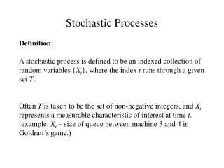
3. Stochastic Process • A stochastic process N= {N(t), t T} is a collection of r.v., i.e., for each t in the index set T, N(t) is a random variable • t: time • N(t): state at time t • If T is a countable set, N is a discrete-time stochastic process • If T is continuous, N is a continuous-time stoc. proc.

4. Counting Process • A stochastic process {N(t) ,t  0} is said to be a counting process if N(t) is the total number of events that occurred up to time t. Hence, some properties of a counting process is • N(t)  0 • N(t) is integer valued • If s < t, N(t)  N(s) • For s < t, N(t) – N(s) equals number of events occurring in the interval (s, t]

5. Counting Process • Independent increments • If the number of events that occur in disjoint time intervals are independent • Stationary increments • If the dist. of number of events that occur in any interval of time depends only on the length of time interval

6. Poisson Process • Def. A: the counting process {N(t), t0} is said to be Poisson process having rate l, l>0 if • N(0) = 0; • The process has independent-increments • Number of events in any interval of length t is Poisson dist. with mean lt, that is for all s, t 0.

7. Poisson Process • Def. B: The counting process {N(t), t 0} is said to be a Poisson process with rate l, l>0, if • N(0) = 0 • The process has stationary and independent increments • P[N(h) = 1] = lh +o(h) • P[N(h)  2] = o(h) • The func. f is said to be o(h) if • Def A  Def B, i.e,. they are equivalent. • We show Def B  Def A • Def A  Def B is HW

8. Important Properties • Property 1: mean number of event for any t 0, E[N(t)]=lt. • Property 2: the inter-arrival time dist. of a Poisson process with rate l is an exponential dist. with parameter l. • Property 3: the superposition of two independent Poisson process with rate l1 and l2 is a Poisson process with rate l1+l2

9. Properties (cont.) • Property 4: if we perform Bernoulli trials to make independent random erasures from a Poisson process, the remaining arrivals also form a Poisson process • Property 5: the time until rth arrival , i.e., tr is known as the rth order waiting time, is the sum of r independent experimental values of t and is described by Erlan pdf.

10. Ex 1 • Suppose that X1 and X2 are independent exponential random variables with respective means 1/l1 and 1/l2;What is P{X1 < X2}

12. Conditional Dist. Of the Arrival Time • Suppose we are told that exactly one event of a Poisson process has taken place by time t, what is the distribution of the time at which the event occurred?

14. Ex 2 • Consider the failure of a link in a communication network. Failures occur according to a Poisson process with rate 4.8 per day. Find • P[time between failures  10 days] • P[5 failures in 20 days] • Expected time between 2 consecutive failures • P[0 failures in next day] • Suppose 12 hours have elapsed since last failure, find the expected time to next failure

16. Markov Process • P[X(tn+1)  Xn+1| X(tn)= xn, X(tn-1) = xn-1,…X(t1)=x1] = P[X(tn+1)  Xn+1| X(tn)=xn] • Probabilistic future of the process depends only on the current state, not on the history • We are mostly concerned with discrete-space Markov process, commonly referred to as Markov chains • Discrete-time Markov chains • Continuous-time Markov chains

17. DTMC • Discrete Time Markov Chain: • P[Xn+1= j | Xn= kn, Xn-1 = kn-1,…X0= k0] = P[Xn+1 = j | Xn= kn] • discrete time, discrete space • A finite-state DTMC if its state space is finite • A homogeneous DTMC if P[Xn+1= j | Xn= i ] does not depend on n for all i, j, i.e., Pij = P[Xn+1= j | Xn= i ], where Pij is one step transition prob.

18. Definition • P = [ Pij] is the transition matrix • A matrix that satisfies those conditions is called a stochastic matrix • n-step transition prob.

19. Chapman-Kolmogorov Eq. • Def. • Proof:

20. Question • We have only been dealing with conditional prob. but what we want is to compute the unconditional prob. that the system is in state j at time n, i.e.

21. Result 1 • For all n  1, pn = p0Pn, where pm = (pm(0),pm(1),…) for all m  0. From the above equ., we deduce that pn+1 = pnP. Assume that limnpn(i) exists for all i, and refer it as p(i). The remaining question is how to compute p • Reachable: a state j is reachable from i. if • Communicate: if j is reachable from i and if i is reachable form j, then we say that i and j communicate (i  j)

22. Result 1 (cont.) • Irreducible: • A M.C. is irreducible if i  j for all i,j I • Aperiodic: • For every state iI, define d(i) to be largest common divisor of all integer n, s.t.,

23. Result 2 • Invariant measure of a M.C., if a M.C. with transition matrix P is irreducible and aperiodic and if the system of equation p=pP and p1=1 has a strict positive solution then p(i) = limnpn(i) independently of initial dist. • Invariant equ. : p=pP • Invariant measure p

24. Gambler’s Ruin Problem • Consider a gambler who at each play of game has probability p of winning one unit and probability q=1-p of losing one unit. Assuming that successive plays of the game are independent, what is the probability that, starting with i units, the gambler’s fortune will reach N before reaching 0?

25. Ans • If we let Xn denote the player’s fortune at time n, then the process {Xn, n=0, 1,2,…} is a Markov chain with transition probabilities: • p00 =pNN =1 • pi,i+1 = p = 1-pi,i-1 • This Markov chain has 3 classes of states: {0},{1,2,…,N-1}, and {N}

26. Let Pi, i=0,1,2,…,N, denote the prob. That, starting with i, the gambler’s fortune will eventually reach N. • By conditioning on the outcome of the initial play of the game we obtain • Pi = pPi+1 + qPi-1, i=1,2, …, N-1 Since p+q =1 Pi+1 – Pi = q/p(Pi-Pi-1), Also, P0 =0, so P2 – P1 = q/p*(P1-P0) = q/p*P1 P3 - P2 =q/p*(P2-P1)= (q/p)2*P1

28. If p > ½, there is a positive prob. that the gambler’s fortune will increase indefinitely • Otherwise, the gambler will, with prob. 1, go broke against an infinitely rich adversary.

29. CTMC • Continuous-time Markov Chain • Continuous time, discrete state • P[X(t)= j | X(s)=i, X(sn-1)= in-1,…X(s0)= i0] = P[X(t)= j | X(s)=i] • A continuous M.C. is homogeneous if • P[X(t+u)= j | X(s+u)=i] = P[X(t)= j | X(s)=i] = Pij[t-s], where t > s • Chapman-Kolmogorov equ.

30. CTMC (cont.) • p(t)=p(0)eQt • Q is called the infinitesimal generator • Proof:

31. Result 3 • If a continuous M.C. with infinitesimal generator Q is irreducible and if the system of equations pQ = 0, and p1=1, has a strictly positive solution then p(i)= limtp(x(t)=i) for all iI, independently of the initial dist.