Stochastic Processes
Stochastic Processes. A stochastic process describes the way a variable evolves over time that is at least in part random. i.e., temperature and IBM stock price


Stochastic Processes
E N D
Presentation Transcript
Stochastic Processes • A stochastic process describes the way a variable evolves over time that is at least in part random. i.e., temperature and IBM stock price • A stochastic process is defined by a probability law for the evolution of a variable xt over time t. For given times, we can calculate the probability that the corresponding values x1,x2, x3,etc. lie in some specified range.
Categorization of Stochastic Processes • Discrete time; discrete variable Random walk: if can only take on discrete values • Discrete time; continuous variable is a normally distributed random variable with zero mean. • Continuous time; discrete variable • Continuous time; continuous variable
Modeling Stock Prices • We can use any of the four types of stochastic processes to model stock prices • The continuous time, continuous variable process proves to be the most useful for the purposes of valuing derivative securities
Markov Processes • In a Markov process future movements in a variable depend only on where we are, not the history of how we got where we are. • We will assume that stock prices follow Markov processes.
Weak-Form Market Efficiency • The assertion is that it is impossible to produce consistently superior returns with a trading rule based on the past history of stock prices. In other words technical analysis does not work. • A Markov process for stock prices is clearly consistent with weak-form market efficiency
Example of a Discrete Time Continuous Variable Model • A stock price follows a Markov process, and is currently at $40. • At the end of 1 year it is considered that it will have a probability distribution of f(40,10) where f(m,s) is a normal distribution with mean m and standard deviation s.
Questions • What is the probability distribution of the stock price at the end of 2 years? • ½ years? • ¼ years? • Dt years? Taking limits we have defined a continuous variable, continuous time process
Variances & Standard Deviations • In Markov processes changes in successive periods of time are independent • This means that variances are additive • Standard deviations are not additive
Variances & Standard Deviations (continued) • In our example it is correct to say that the variance is 100 per year. • It is strictly not correct to say that the standard deviation is 10 per year.
A Wiener Process (Brownian Motion) • We consider a variable z whose value changes continuously • The change in a small interval of time Dt is Dz • The variable follows a Wiener process if 1. 2. The values of Dz for any 2 different (non-overlapping) periods of time are independent
Properties of a Wiener Process • Mean of [z (T ) – z (0)] is 0 • Variance of [z (T ) – z (0)] is T • Standard deviation of [z (T ) – z (0)] is
Taking Limits . . . • What does an expression involving dz and dt mean? • It should be interpreted as meaning that the corresponding expression involving Dz and Dt is true in the limit as Dt tends to zero • In this respect, stochastic calculus is analogous to ordinary calculus
Generalized Wiener Processes • A Wiener process has a drift rate (ie average change per unit time) of 0 and a variance rate of 1 • In a generalized Wiener process the drift rate & the variance rate can be set equal to any chosen constants
Generalized Wiener Processes(continued) The variable x follows a generalized Wiener process with a drift rate of a & a variance rate of b2 if dx=adt+bdz or: x(t)=x0+at+bz(t)
Generalized Wiener Processes(continued) • Mean change in x in time T is aT • Variance of change in x in time T is b2T • Standard deviation of change in x in time T is
The Example Revisited • A stock price starts at 40 & has a probability distribution of f(40,10) at the end of the year • If we assume the stochastic process is Markov with no drift then the process is dS = 10dz • If the stock price were expected to grow by $8 on average during the year, so that the year-end distribution is f(48,10), the process is dS = 8dt + 10dz
Why ?(1) • It’s the only way to make the variance of (xT-x0)depend on T and not on the number of steps. 1.Divide time up into n discrete periods of length △t, n=T/ △ t. In each period the variable x either moves up or down by an amount △ h with the probabilities of p and q respectively.
Why ?(2) 2.the distribution for the future values of x: E(△x)=(p-q) △ h E[(△ x)2]= p(△ h)2+q(- △ h)2 So, the variance of △ x is: E[(△ x)2]-[E(△x)]2=[1-(p-q)2](△ h)2=4pq(△ h)2 3. Since the successive steps of the random walk are independent, the cumulated change(xT-x0)is a binomial random walk with mean: n(p-q) △ h=T(p-q) △ h/ △ t and variance: n [1-(p-q)2](△ h)2=4pqT(△ h)2 / △ t
Why ?(3) • When let △t go to zero, we would like the mean and variance of (xT-x0) to remain unchanged, and to be independent of the particular choice of p,q, △ h and △ t. • The only way to get it is to set: and then
Why ?(4) • When △t goes to zero,the binomial distribution converges to a normal distribution, with mean and variance
Sample path(a=0.2 per year,b2=1.0 per year) • Taking a time interval of one month, then calculating a trajectory for xt using the equation: A trend of 0.2 per year implies a trend of 0.0167 per month. A variance of 1.0 per year implies a variance of 0.0833 per month, so that the standard deviation in monthly terms is 0.2887. See Investment under uncertainty, p66
Forecast using generalized Brownian Motion • Given the value of x(t)for Dec. 1974,X1974 , the forecasted value of x for a time T months beyond Dec. 1974 is given by: See Investment under uncertainty, p67 • In the long run, the trend is the dominant determinant of Brownian Motion, whereas in the short run, the volatility of the process dominates.
Why a Generalized Wiener Processes not Appropriate for Stocks • For a stock price we can conjecture that its expected proportional change in a short period of time remains constant not its expected absolute change in a short period of time • The price of a stock never fall below zero.
Ito Process • In an Ito process the drift rate and the variance rate are functions of time dx=a(x,t)dt+b(x,t)dz or: • The discrete time equivalent is only true in the limit as Dt tends to zero
An Ito Process for Stock Prices where m is the expected return s is the volatility. The discrete time equivalent is
Monte Carlo Simulation • We can sample random paths for the stock price by sampling values for e • Suppose m= 0.14, s= 0.20, and Dt = 0.01, then
Ito’s Lemma • If we know the stochastic process followed by x, Ito’s lemma tells us the stochastic process followed by some function G (x, t ) • Since a derivative security is a function of the price of the underlying & time, Ito’s lemma plays an important part in the analysis of derivative securities
Taylor Series Expansion • A Taylor’s series expansion of G(x , t ) gives
Ito’s Lemma for several Ito processes • Suppose F=F(x1,x2,…,xm,xt) is a function of time and of the m Ito process x1,x2,…,xm, where dxi=ai(x1,x2,…,xm,t)dt+bi(x1,x2,…,xm,t)dzi,i=1,…,m,with E(dzidzj)= ρijdt.Then Ito’s Lemma gives the defferential dF as
Examples Suppose F(x,y)=xy, where x and y each follow geometric Brownian motions: dx=axxdt+bxxdzx dy=ayydt+byydzy with E(dzxdzy)=ρdt. What’s the process followed by F(x,y) and by G=logF? dF=xdy+ydx+dxdy =(ax+ay+ ρbxby)Fdt+(bxdzx+bydzy)F dG= (ax+ay-1/2bx2-1/2by2)dt+bxdzx+bydzy