Testing a Claim
Testing a Claim. Chapter 11. 1.1 Intro. “I can make 80% of my BBall free throws”. To test my claim, you ask me to shoot 20 free throws. I only make 8 and you say “aha! Someone who makes 80% of their free throws would NEVER only make 8/20!”


Testing a Claim
E N D
Presentation Transcript
Testing a Claim Chapter 11
1.1 Intro • “I can make 80% of my BBall free throws”. To test my claim, you ask me to shoot 20 free throws. I only make 8 and you say “aha! Someone who makes 80% of their free throws would NEVER only make 8/20!” • But I say, ‘hey, what if I’m having a bad day, or am injured, or the ball is dead, or the hoop is bent…” Since all of these are possibilities, you say “OK, well I’ll decide how likely your claim is based on the probability that someone who genuinely makes 80% would shoot 8/20 on one trial run” • This is the basics of hypothesis testing: an outcome that would rarely happen if a claim were true is good evidence that the claim is not true.
Stating a hypothesis • A statistical test starts with a careful statement of the claims we want to compare. Because the reasoning of tests look for evidence against a claim, we start with the claim we seek evidence AGAINST. • This is called our NULL HYPOTHESIS. (H0) • The claim about the population we are trying to find evidence FOR is our ALTERNATIVE hypothesis (HA)
Example (one-sided) • Attitudes towards school and study habits on a national survey range from 0 to 200. The mean score for US college students is 115 with a standard deviation of 30. Assume normality in this population. A teacher suspects that older students have better attitudes towards school. She gives the survey to a SRS of 25 students. • We seek evidence AGAINST the claim that μ = 115. • Null: H0: • Alternate: Ha: • *Be sure to state the hypothesis in terms of population b/c we are making inference/claims about our pop!
Two sided hypothesis • If the previous example said the teacher thought that seniors had a DIFFERENT attitude towards study habits (but didn’t specify better or worse), we would be doing a two sided hypothesis because the alternate is that μ could be > or < 115. So we state it as: • H0: • Ha: • **The alternative hypothesis should express the hopes or suspicions we have before we see the data. It is cheating to first look at the data and then frame Ha to fit what the data show!
Conditions for Significance tests • The same 3 conditions from Chapter 10 should be verified before performing a significance test about a population mean or proportion. • 1. SRS • 2. Normality: • Means ( known) -> CLT • Means (unknown) n<15, n≥15, n≥ 30 • Proportions np≥ 10 and n(1 – p) ≥ 10 • 3. Independence: N≥10n and/or individual observations are independent
Test Statistic • The significance test compares the value of the parameter (true pop mean, as stated in the null) with the calculated sample mean. Values of the sample far from the true parameter give evidence against H0 • To assess how far the sample statistic is from the population parameter, we have to standardize it (to make comparison) • Test statistic =
Z test Attitudes towards school and study habits on a national survey range from 0 to 200. The mean score for US college students is 115 with a standard deviation of 30. Assume normality in this population. A teacher suspects that older students have better attitudes towards school. She gives the survey to a SRS of 25 students. • We will focus on the Z test first, which is when we know sigma, so the Z test statistic formula is: • In that last example, lets say the mean (X bar) of the 25 seniors sampled was 125. Our calculated Z would be • Test statistic =
A South Florida newspaper reports that the average cost of renting a car in Fort Lauderdale during the months of January and February is $36 per day. A random sample was taken of 40 people who rented cars at Fort Lauderdale Airports and the mean of this sample was found to be = $34.20. The population standard deviation is known to be We want to test the claim that the average rental in Fort Lauderdale is less than that reported by the newspaper. • Which of the following would be the correct test statistic? (a) 0.0636 (b) -0.0636 (c) 0.127 (d) -0.045
P-Value • We use our test statistic to calculate our p-value • The p value is the probability of getting your observed statistic, assuming the null is true. • Small p-value = reject our Null Hypothesis • The p value is the area under the curve from your calculated test statistic, to the tail end. For Example: • Test statistic = 1.67 • Null: H0: μ= 115 • Alternate: Ha: μ> 115
P-Value • The p value is the area under the curve from your calculated test statistic, to the tail end. • Be careful if you are performing a two-sided test!!! For Example: • Test statistic = 1.67 • Null: H0: μ= 115 • Alternate: Ha: μ ≠ 115
In a test of H0: p = 0.7 against Ha: p ≠ 0.7, a sample size of 80 produces z = 0.8 for the value of the test statistic. Which of the following is closes to the P-value of the test?
Interpretation: Statistical Significance • We set a “maximum” p-value before calculating our observed test statistic and we call this our significance level. • is the symbol for our chosen significance level we need to beat. So we would say =.05 • Most commonly we choose=.05 • meaning we need our calculated p value to be less than .05,
If we “beat” our alpha level – Reject H0 • If we do not “beat” our alpha level -- fail to reject H0
If our calculated (or observed) p-value is less than or equal to our alpha level, we say that the data is “statistically significant at level α” • When our data is statistically significant, we can reject our null hypothesis. • “significant” doesn’t mean important! It just means you are rejecting your null hypothesis
Inference Toolbox! • To test a claim about an unknown population parameter: • Step 1: State • Identify the parameter (in context) and state your hypotheses • Step 2: Plan • Identify the appropriate inference procedure andverify the conditions for using it (SRS, Normality, Independence) • Step 3: Calculations • Calculate the test statistic • Find the p-value • Step 4: Interpretation • Interpret your results in CONTEXT • Interpret P-value or make a decision about H0 using statistical significance
Example =) • Mel N. Colly is interested in whether or not his new treatment for depressed patients is having any effect on his patients’ rating of depression. Suppose all of his depressed patients have a mean depression score of 8 with a standard deviation of 4. Mel chooses a random sample of 100 depressed patients treated with his innovative approach and determines that the mean depression score for these individuals is 7.5. Does the cream have any effect?
Mel N. Colly is interested in whether or not his new treatment for depressed patients is having any effect on his patients’ rating of depression. Suppose all of his depressed patients have a mean depression score of 8 with a standard deviation of 4. Mel chooses a random sample of 30 depressed patients treated with his innovative approach and determines that the mean depression score for these individuals is 7.5. Does the treatment have any effect? • Step 1: STATE • We are interested in the true mean depression score of all of Mel’s depressed patients • H0 : • HA :
Mel N. Colly is interested in whether or not his new treatment for depressed patients is having any effect on his patients’ rating of depression. Suppose all of his depressed patients have a mean depression score of 8 with a standard deviation of 4. Mel chooses a random sample of 30 depressed patients treated with his innovative approach and determines that the mean depression score for these individuals is 7.5. Does the treatment have any effect? • Step 2: PLAN • We will conduct a ______________________________. • (1) SRS: • The data was collected “at random.” The study does not state that a simple random sample was used, but we will proceed assuming proper sampling methods were used. • (2) Normality: • We do not know if the population distribution of depression patients’ depression scores is Normal, but the sample size is large enough (n=30) so that the sampling distribution will be approximately normal (by the central limit theorem) • (3) Independence: • Mel N. Colly selected the patients without replacement, but we will assume that there are more than 30(10) = 300 depressed patients seen in his practice.
Mel N. Colly is interested in whether or not his new treatment for depressed patients is having any effect on his patients’ rating of depression. Suppose all of his depressed patients have a mean depression score of 8 with a standard deviation of 4. Mel chooses a random sample of 30 depressed patients treated with his innovative approach and determines that the mean depression score for these individuals is 7.5. Does the treatment have any effect? • Step 3: Calculations • (1) Test Statistic z =x-bar - μ0 σ/√n • (2) P-value: Draw a picture using the standardized value, then calculate the P-value
Mel N. Colly is interested in whether or not his new treatment for depressed patients is having any effect on his patients’ rating of depression. Suppose all of his depressed patients have a mean depression score of 8 with a standard deviation of 4. Mel chooses a random sample of 30 depressed patients treated with his innovative approach and determines that the mean depression score for these individuals is 7.5. Does the treatment have any effect? • Step 4: Interpretation • P-value (the problem did not give us an alpha level) • A sample mean depression score of 7.5 would happen 49.36% of the time by chance if the true population mean depression score was 8. Because the probability of obtaining these results is so high, this is not good evidence that the true mean depression score is not 8.
Di Perrs is the quality control manager for Pampers. Pampers claims the average absorbency of Pampers is 195 milliliters with a standard deviation of 80 milliliters. A sample of 100 Pampers were selected at random and tested. The average amount of fluid absorbed was x-bar = 210 milliliters. Di Perrs wants to use an α = 0.05 significance level to determine whether or not the company’s claim is true. • Step 1: STATE • We are interested in the true mean absorbency in ml of all Pampers. • H0 : • HA:
Step 2: PLAN • We will perform a 1-sample z-test for means (sigma known) • (1) SRS: The data was collected “at random.” The study does not state that a simple random sample was used, but we will proceed assuming proper sampling methods were used. • (2) Normality: We do not know if the population distribution of Pampers absorbency is Normal, but the sample size is large enough (n=100) so that the sampling distribution will be approximately normal (by the central limit theorem) • (3) Independence: Di Perrs selected the diapers without replacement, but we can assume that there are more than 10(100) = 1000 diapers produced at the factory.
Di Perrs is the quality control manager for Pampers. A recent ad claimed that the new improved Pampers is more absorbent than the old Pampers. The average absorbency of old pampers was 195 milliliters with a standard deviation of 80 milliliters. A total of 100 new Pampers were selected at random and tested. The average amount of fluid absorbed was x-bar = 210 milliliters. Di Perrs wants to use an α = 0.05 significance level. • Step 3: Calculations • (1) Test Statistic • (2) P-value: Draw a picture using the standardized value, then calculate the P-value
Di Perrs is the quality control manager for Pampers. A recent ad claimed that the new improved Pampers is more absorbent than the old Pampers. The average absorbency of old pampers was 195 milliliters with a standard deviation of 80 milliliters. A total of 100 new Pampers were selected at random and tested. The average amount of fluid absorbed was x-bar = 210 milliliters. Di Perrs wants to use an α = 0.05 significance level. • Step 4: Interpretation • Using significance Level • Since our P-value,
Prom • Worried about his prospects for the prom, Malcolm claims that girls at NPHS are a bit snobby and that the average number of girls that a guy must ask to the prom before getting a “yes” is 4. • Doug disagrees. He doesn’t think the girls are that snobby and that the average number of girls that a guy must ask out before getting a positive response is less than 4. • An SRS from last year of 50 junior and senior guys found that the average number of girls that a guy asked out to the prom was 3.4. Assuming the standard deviation from the entire population is, is there enough evidence to support Alex’s claim (at the level?)