Chapter 11 Testing a Claim
Chapter 11 Testing a Claim. AP Statistics Hamilton/Mann. Introduction. Confidence intervals are one of the two most common types of statistical inference. Use confidence intervals when you want to estimate a population parameter.


Chapter 11 Testing a Claim
E N D
Presentation Transcript
Chapter 11Testing a Claim AP Statistics Hamilton/Mann
Introduction • Confidence intervals are one of the two most common types of statistical inference. • Use confidence intervals when you want to estimate a population parameter. • The second common type of statistical inference, called significance tests, has a different goal: to assess the evidence provided by data about some claim concerning a population. • The following example will help us to understand the reasoning of statistical tests.
I’m a Great Free-Throw Shooter! • I claim that I make 80% of my free throws. To test my claim, you ask me to shoot 20 free throws. I only make 8 of the 20 free throws and you believe you have disproven me and say, “Someone who makes 80% of their free throws would almost never make only 8 out of 20. So I don’t believe your claim.” • Your reasoning is based on asking what would happen if my claim were true and we repeated the sample of 20 free throws many times – I would almost never make as few as 8. This event is so unlikely that it gives strong evidence that my claim is not true.
I’m a Great Free-Throw Shooter! • You can say how strong the evidence against my claim is by giving the probability that I would make as few as 8 out of 20 shots if I really were an 80% free throw shooter. That probability is 0.0001. (How’d we get that?) I would make 8 free throws or less only once in 10,000 tries in the long run if my claim to make 80% is true. • This small probability convinces you that I am lying. • Significance tests use an elaborate vocabulary, but the idea is simple: an outcome that would rarely happen if a claim were true is good evidence that the claim is not true.
Chapter 11 Section 1 Significance Tests: The Basics HW: 11.3, 11.4, 11.5, 11.6, 11.7, 11.8, 11.11, 11.12, 11.14, 11.16…due Tuesday at the end of class
Significance Tests Background • A significance test is a formal procedure for comparing observed data with a hypothesis whose truth we want to assess. • The hypothesis is a statement about a population parameter, like the population mean or population proportion p. • The results of the test are expressed in terms of a probability that measures how well the data and the hypothesis agree. • The reasoning of statistical tests, like that of confidence intervals, is based on asking what would happen if we repeated the sampling or experiment many times. • We will begin by unrealistically assuming that we know the population standard deviation
Call the Paramedics • Vehicle accidents can result in serious injury to drivers and passengers. When they do, people generally call 911. Emergency personnel then report to these emergency calls as quickly as possible. Slow response times can have serious consequences for accident victims. In case of life-threatening injuries, victims generally need medical attention within 8 minutes of the crash. • For this reason several cities have begun monitoring paramedic response times.
Call the Paramedics • In one such city, the mean response time to all accidents involving life-threatening injuries last year was minutes with a standard deviation of minutes. The city manager shares this information with emergency personnel and encourages them to “do better” next year. • At the end of the next year, the city manager selects an SRS of 400 calls involving life-threatening injuries and examines the response times. For this sample, the mean response time was minutes. Do these data provide good evidence that response times have decreased since last year?
What do we think? • Remember, sample results vary! Maybe the response times have not improved at all and the apparent improvement is a result of sampling variability. • We are going to make a claim and ask if the data gives evidence against it. We would like to conclude that the mean response time has decreased, so the claim we test is that response times have not decreased. For that claim, the mean response time of all calls involving life-threatening injuries would be minutes. We will also assume that minutes for this year’s calls too.
What do we think? (cont.) • If the claim that minutes is true, the sampling distribution of from 400 calls will be approximately Normal (by the CLT) with mean minutes and standard deviation minutes. We can judge whether any observed value is unusual by locating it on this distribution. • Is a value of 6.48 for unusual? • Is a value of 6.61 for unusual?
What do we think? (cont.) • The city manager’s observed value of 6.48 is far from the distribution’s mean of minutes. In fact, it so far that it would rarely occur by chance if the mean was minutes. This observed value is good evidence that the true mean is less than 6.7 minutes. In other words, it appears that the average response time did decrease this year, and the paramedics should be commended for a job well done. • This outlines the reasoning of significance tests.
Stating Hypotheses • A statistical test starts with a careful statement of the claims that we want to compare. In our prior example, we asked if the accident response time data were likely if, in fact, there is no decrease in paramedics’ response times. • Because the reasoning of tests looks for evidence against a claim, we start with the claim we seek evidence against, such as “no decrease in response time.” This claim is our null hypothesis.
We abbreviate the null hypothesis as H0 and the alternative hypothesis as Ha. In our example, we were seeking evidence of a decrease in response time this year. For this reason, the null hypothesis would say that there was “no decrease” and the alternative hypothesis would say that “there was a decrease.” The hypotheses are
Stating Hypotheses • Since we were only interested in the fact that the mean time had decreased, the alternative hypothesis is one-sided. • Hypotheses always refer to some population, not to a particular outcome. So always state H0 and Ha in terms of a population parameter. • Because Ha expresses the effect that we hope to find evidence for, it is often easier to begin by stating Ha and then setting up H0 as the statement that the hoped-for effect is not present.
Studying Job Satisfaction • Does the job satisfaction of assembly workers differ when their work is machine-paced rather than self-paced? One study chose 18 workers at random from a group of people who assembled electronic devices. Half the subjects were assigned at random to each of the two groups. Both groups did similar assembly work, but one work setup allowed workers to pace themselves, and the other featured an assembly line that moved at fixed time intervals so that the workers were paced by the machine. After two weeks, all subjects took the Job Diagnosis Survey (JDS), a test of job satisfaction. Then they switched work setups and took the JDS again after two more weeks.
Studying Job Satisfaction (cont.) • This is a matched pairs design. The response variable is the difference in the JDS scores, self-paced minus machine-paced. The parameter of interest is the mean of the differences in JDS scores in the population of all assembly workers. • Since we are asking “Does the job satisfaction of assembly workers differ when their work is machine-paced rather than self-paced?,” our alternative hypothesis will be that the job satisfaction does differ. If they were the same, then the mean difference would be 0. • since difference means they aren’t equal.
Studying Job Satisfaction (cont.) • The alternative hypothesis should express the hopes or suspicions we have before we see the data. It is cheating to first look at the data and then frame Ha to fit what the data show.
Conditions for Significance Tests • To create a confidence interval we had to have: • an SRS from the population of interest • Normality • independent observations • These are the same three conditions for a significance test. • The details for checking the Normality condition for means and proportions are different. • For means – population is Normal or large sample size • For proportions -
Checking Conditions on Call the Paramedics • Before conducting a significance test about the mean response time of paramedics, we should check our conditions. • SRS – We were told that the city manager took an SRS of 400 calls involving life-threatening injuries. • Normality – The population distribution of paramedic response times may not follow a Normal distribution, but our sample size (400) is large enough to ensure that the sampling distribution of is approximately Normal (by the Central Limit Theorem). • Independence – We must assume that there were at least 4000 calls that involved life-threatening injuries for the observations to be independent. • We appear to meet all three conditions.
Test Statistics • A significance test uses data in the form of a test statistic. Here are some principles that apply to most tests: • The test is based on a statistic that compares the value of the parameter as stated in the null hypothesis with an estimate of the parameter from the sample data. • Values of the estimate far from the parameter value in the direction specified by the alternative hypothesis give evidence against H0. • To assess how far the estimate is from the parameter, standardize the estimate. In many common situations, the test statistic has the form
Call the Paramedics (cont.) • For this example, the null hypothesis was and the estimate of was minutes. Since we were assuming that minutes for the distribution of response times, our test statistic is where is the value of specified in the null hypothesis. The test statistic z says how far is from in standard deviation units.
Call the Paramedics (cont.) • So, for our example, • Because this sample result is over two standard deviations below the hypothesized mean of 6.7, it gives good evidence that the mean response time this year is not 6.7 minutes, but rather, less than 6.7 minutes.
P-values • The null hypothesis H0 states the claim we are seeking evidence against. The test statistic measures how much the sample data diverge from the null hypothesis. If the test statistic is large and is in the direction suggested by the alternative hypothesis Ha, we have data that would be unlikely if H0 were true. We make “unlikely” precise by calculating a probability, called a P-value.
P-values • Small P-values are evidence against H0 because they say that the observed result is unlikely to occur when H0 is true. Large values fail to give evidence against H0.
Call the Paramedics (cont.) • Recall that our test statistic had the value • Since the alternative hypothesis Ha was a negative z-value would favor Ha over H0. • The P-value is the probability of getting a sample result that is at least as extreme as the one we did if H0 were true. In other words, the P-value is calculated assuming that
Call the Paramedics (cont.) • So • The shaded area under the curve is the P-value of the sample results
Call the Paramedics (cont.) • So there is about a 1.4% chance that the city manager would select a sample of 400 calls with a mean of 6.48 minutes or less. • This small P-value provides strong evidence against H0 and in favor of the alternative • For this reason, we believe that there is evidence to suggest that the mean response times of the paramedics to accidents that produced life-threatening injuries has decreased.
Job Satisfaction • Recall that our hypotheses for job satisfaction were • Suppose we know that the differences in job satisfaction follow a Normal distribution with a standard deviation of • Data from 18 workers gave that is these workers preferred the self-paced environment on average. • The test statistic is
Job Satisfaction (cont.) • Because the alternative hypothesis is two-sided, the P-value is the probability of getting at least as far from 0 in either direction as the observed z = 1.20. As always, calculate the P-value by taking H0 to be true. When H0 is true, and z has a standard Normal distribution. • So we are looking for • Since values as far from 0 as would occur approximately 23% of the time when the mean is it is not good evidence that there is a difference in job satisfaction.
Statistical Significance • We sometimes take one final step to assess the evidence against H0. We can compare the P-value with a fixed value that we regard as decisive. This amounts to announcing in advance how much evidence against H0 we will insist on. This decisive value of P is called the significance level. • We write it as α, the Greek letter alpha. If we choose α = 0.05, we are requiring that the data give evidence against H0 so strong that it would happen no more than 5% of the time when H0 is true. If we choose α = 0.01, we are insisting on stronger evidence against H0, evidence so strong that it would appear only 1% of the time if H0 is true.
Significant in the statistical sense does not mean important. It simply means “not likely to happen by chance.” The significance level α makes “not likely” more precise. Significance at level 0.01 is often expressed by the statement “The results were significant (P < 0.01).” Here the P stands for the P-value. The P-value is more informative than a statement of significance because it allows us to assess significance at any level we choose. For example, a result with P=0.03 is significant at the α = 0.05 level, but is not significant at the α = 0.01 level.
Paramedic Response Times • We found that the P-value for paramedic response times was 0.0139. This result is statistically significant at the α = 0.05 level since 0.0139<0.05, but is not significant at the α = 0.01 level because The figure below gives a visual representation of this relationship.
Significance Levels • In practice, the most commonly used significance level is α = 0.05. • Sometimes it may be preferable to choose α = 0.01 or α = 0.10, for reasons we will discuss later.
Interpreting Results in Context • The final step is to draw a conclusion about the competing claims you were testing. As with confidence intervals, the conclusion should have a clear connection to your calculations and should be stated in the context of the problem. In significance testing there are two acceptable methods for drawing conclusions: • One based on P-values • One based on statistical significance • Both methods describe the strength of the evidence against the null hypothesis H0.
Interpreting Results in Context • We have already seen an example of the P-value approach. • Our other option is to make one of two decisions about the null hypothesis H0 based on whether or result is statistically significant. • Reject H0 – There is sufficient evidence to believe the null hypothesis is incorrect • Fail to reject H0 – There is not sufficient evidence to believe that the null hypothesis is incorrect. This does not mean that it is correct, just that we cannot show that it is not incorrect.
Interpreting Results in Context • We reject H0 if our sample result is too unlikely to have occurred by chance assuming H0 is true. In other words, we will reject H0 if our result is statistically significant at the given α level. • If our sample result could possibly have happened by chance assuming H0 is true, we will fail to reject H0. That is, we will fail to reject H0 if our result is not significant at the given α level. • We should always interpret the results by remembering the three C’s: conclusion, connection, and context.
Paramedics (cont.) • The P-value for the city manager’s study of response times was P = 0.0139. If we were using an α = 0.05 significance level, we would reject minutes (conclusion) since our P-value is less than our significance level α = 0.05 (connection). In other words, it appears that the mean response time to all life-threatening calls this year is less than last year’s average of 6.7 minutes (context).
Job Satisfaction (cont.) • The P-value for the job satisfaction study was P = 0.2302. If we were using an α = 0.05 significance level, we would fail to reject (conclusion) since our P-value is greater than our significance level α = 0.05 (connection). In other words, it is possible that the mean difference in job satisfaction scores for workers in a self-paced versus machine-paced environment is 0 (context).
Final Notes • If you are going to draw a conclusion based on statistical significance, the significance level α should be selected before the data are produced to prevent manipulating the data. • A P-value is more informative than a “reject” or “fail to reject” conclusion at a given significance level. The P-value is the smallest α level at which the data are significant. • Knowing the P-value allows us to assess significance at any level. • However, interpreting the P-value is more challenging than making a decision about H0 based on statistical significance.
Chapter 11 Section 2 Carrying Out Significance Tests HW: 11.27, 11.28, 11.30, 11.31, 11.32, 11.33, 11.34
Inference Toolbox Reminder • To test a claim about an unknown population parameter: • Step 1: Hypotheses – Identify the population of interest and the parameter you want to draw conclusions about. State hypotheses. • Step 2: Conditions – Choose the appropriate inference procedure and verify the conditions for using it. • Step 3: Calculations – If the conditions are met, carry out the inference procedure. • Calculate the test statistic. • Find the P-value. • Step 4: Interpretation – Interpret your results in the context of the problem. • Interpret the P-value or make a decision about H0 using statistical significance. • Don’t forget the three C’s: conclusion, connection, and context.
Once you have completed the first two steps, a calculator or computer can do Step 3. Here is the calculation step for carrying out a significance test about the population mean μ in the unrealistic setting when σ is known.
Executives’ Blood Pressures • The medical director of a large company is concerned about the effects of stress on the company’s younger executives. According to the National Center for Health Statistics, the mean systolic blood pressure for males 35 to 44 years of age is 128, and the standard deviation in this population is 15. The medical director examines the medical records of 72 male executives in this age group and finds that their mean systolic blood pressure is Is this evidence that the mean blood pressure for all the company’s younger male executives is different from the national average?
Executives’ Blood Pressures (cont.) • Step 1 – The population of interest is all male executives aged 35 to 44 at this company. The parameter of interest is the mean systolic blood pressure μ of these male executives aged 35 to 44. Since we want to check that the mean blood pressure is different, the alternative hypothesis would be that it is different from, in other words, not equal to, the national average of 128 for men in this age group. So, the null hypothesis would be that the mean systolic blood pressure would be the same as the national average.
Executives’ Blood Pressures (cont.) • Step 2 – Conditions • SRS – We are not told. If the records that are being checked are not an SRS, then our results may be questionable. For instance, if we only have records for executives who have been ill, this introduces bias because illness is usually accompanied by higher blood pressure. • Normality – The sample is large enough (72) for the Central Limit Theorem to tell us that the sampling distribution of is approximately Normal. • Independence – We must assume that there are at least 720 executives aged 35 to 44 who work for this large company. If not, independence does not hold.
Executives’ Blood Pressures (cont.) • Step 3 – Calculations • Since the test is two-sided, we have to find the probability that we are less than -1.09 or greater than 1.09. • Step 4 – Conclusions – Since our P-value is 0.2758, we fail to reject the null hypothesis that Therefore, there is not good evidence that the mean systolic blood pressure of the male executives aged 35 to 44 differs from the national average.
Executives’ Blood Pressures (cont.) • The data for our example do not establish that the mean systolic blood pressure μ for the male executives aged 35 to 44 is 128. We sought evidence that μ differed from 128 and failed to find convincing evidence. That is all we can say. • Most likely, the mean systolic blood pressure of all male executives aged 35 to 44 is not exactly equal to 128. A large enough sample would give evidence of the difference, even if it is very small. • Failing to find evidence against H0 means only that the data are consistent with H0, not that we have clear evidence that H0 is true.
Health Promotion Program • The company medical director initiated a health promotion campaign to encourage employees to exercise more and eat a healthier diet. One measure of the effectiveness of such a program is a drop in blood pressure. The director chooses a random sample of 50 employees and compares their blood pressures from physical exams given before the campaign and again a year later. The mean change in systolic blood pressure for these 5o employees is We assume that the population standard deviation is The director wants to use an significance level.