Basic concept
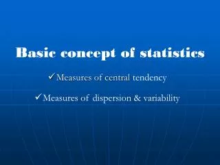
Basic concept. Measures of central tendency. Measures of dispersion & variability. Measures of tendency central. Arithmetic mean (= simple average ). Best estimate of population mean is the sample mean, X. measurement in population. summation. sample size. index of measurement.

Basic concept
E N D
Presentation Transcript
Basic concept • Measures of central tendency • Measures of dispersion & variability
Measures of tendency central Arithmetic mean (= simple average) • Best estimate of population mean is the sample mean, X measurement in population summation sample size index of measurement
Measures of variability • All describe how “spread out” the data are. • Sum of squares,sum of squared deviations from the mean • For a sample,
Why? • Average or mean sum of squares = variance, s2: • For a sample,
n – 1 represents the degrees of freedom, , or number of independent quantities in the estimate s2. Greek letter “nu” • therefore, once n – 1 of all deviations are specified, the last deviation is already determined.
Standard deviation, s • Variance has squared measurement units – to regain original units, take the square root … • For a sample,
Standard error of the mean • Standard error of the mean is a measure of variability among the means of repeated samples from a population. • For a sample,
Means of repeated random samples, each with sample size, n = 5 values … A Population of Values 14 15 13 14 14 13 12 16 14 14 14 16 13 14 14 13 12 14 13 14 13 16 14 13 14 15 15 16
For a large enough number of large samples, the frequency distribution of the sample means (= sampling distribution), approaches a normal distribution.
Testing statistical hypotheses between 2 means • State the research question in terms of statistical hypotheses. • We always start with a statement that hypothesizes “no difference”, called the null hypothesis = H0. • E.g., H0: Mean bill length of female hummingbirds is equal to mean bill length of male hummingbirds, µ=µ.
Then we formulate a statement that must be true if the null hypothesis is false, called the alternate hypothesis = HA . • E.g., HA: Mean bill length of female hummingbirds is not equal to mean bill length of male hummingbirds, µµ . • If we reject H0 as a result of sample evidence, then we conclude that HA is true.
Choose an appropriate statistical test that would allow you to reject H0 if H0 were false.
William Sealey Gosset (a.k.a. “Student”) E.g., Student’s t test for hypotheses about means
Is the difference between sample means bigger than we would expect, given the variability in the sampled populations?
Mean of sample 1 Mean of sample 2 Standard error of the difference between the sample means • To estimate s(X1—X2), we must first know the relation between both populations. t Statistic,
Relation between populations • Dependent population • Independent population • Identical (homogenous ) variance • Not identical (heterogeneous) variance
Independent Population with homogenous variances • Pooled variance: • Then,
Select the level of significance for the statistical test. • Level of significance = alpha value = = the probability of incorrectly rejecting the null hypothesis when it is, in fact, true.
Traditionally, researchers choose = 0.05. • 5 percent of the time, or 1 time out of 20, the statistical test will reject H0 when it is true. • Note: the choice of 0.05 is arbitrary!
Determine the critical value the test statistic must attain to be declared significant. • Most test statistics have a frequency distribution …
When sample sizes are small, the sampling distribution is described better by the t distribution than by the standard normal (Z) distribution. • Shape of t distribution depends on degrees of freedom, = n – 1.
Z = t(=) t(=25) t(=5) t(=1) t
The distribution of a test statistic is divided into an area of acceptance and an area of rejection.
For = 0.05 0.025 0.95 0.025 Area of Acceptance Area of Rejection Area of Rejection 0 Lower critical value Upper critical value t
E.g., Mean bill length from a sample of 5 female hummingbirds, X1 = 15.75; • Mean bill length from a sample of 5 male hummingbirds, X2 = 14.25; • Perform the statistical test.
Compare the calculated test statistic with the critical test statistic at the chosen . • Draw and state the conclusions. • Reject or fail to reject H0. • Obtain the P-value = probability for the test statistic.
E.g., to test H0: µ = µ, HA: µ µat = 0.05 using n= 5, n = 5, t(2), = t0.05(2),8 = 2.306. , if |t| 2.306, reject H0.
Since calculated t > t0.05(2),8 (because 3.000 > 2.306), reject H0. • Conclude that hummingbird bill length is sexually size-dimorphic.
What is the probability, P, of observing by chance a difference as large as we saw between female and male hummingbird bill lengths? 0.01 < P < 0.02
Analysis of Variance (ANOVA)
What is ANOVA? • ANOVA (Analysis of Variance) is a procedure designed to determine if the manipulation of one or more independent variables in an experiment has a statistically significant influence on the value of the dependent variable. • It is assumed • Each independent variable is categorical (nominal scale). Independent variables are called Factors and their values are called levels. • The dependent variable is numerical (ratio scale) • The basic idea is that the “variance” of the dependent variable given the influence of one or more independent variables {Expected Sum of Squares for a Factor} is checked to see if it is significantly greater than the “variance” of the dependent variable (assuming no influence of the independent variables) {also known as the Mean-Square-Error(MSE)}.
Analysis of Variance • Analysis of Variance(ANOVA) can be used to test for the equality of three or more population means using data obtained from observational or experimental studies. • We want to use the sample results to test the following hypotheses. H0: 1=2=3=. . . = k Ha: Not all population means are equal • If H0 is rejected, we cannot conclude that all population means are different. • Rejecting H0 means that at least two population means have different values.
Assumptions for Analysis of Variance • For each population, the response variable is normally distributed. • The variance of the response variable, denoted2, is the same for all of the populations. • The effect of independent variable is additive • The observations must be independent.
Analysis of Variance:Testing for the Equality of K Population Means • Between-Treatments Estimate of Population Variance • Within-Treatments Estimate of Population Variance • Comparing the Variance Estimates: The F Test • ANOVA Table
Between-Treatments Estimate of Population Variance • A between-treatments estimate of σ2 is called the mean square due to treatments(MSTR). • The numerator of MSTR is called the sum of squares due to treatments(SSTR). • The denominator of MSTR represents the degrees of freedom associated with SSTR.
Within-Treatments Estimate of Population Variance • The estimate of2based on the variation of the sample observations within each treatment is called the mean square due to error(MSE). • The numerator of MSE is called the sum of squares due to error(SSE). • The denominator of MSE represents the degrees of freedom associated with SSE.
Comparing the Variance Estimates: The F Test • If the null hypothesis is true and the ANOVA assumptions are valid, the sampling distribution of MSTR/MSE is an F distribution with MSTR d.f. equal to k - 1 and MSE d.f. equal to nT - k. • If the means of the k populations are not equal, the value of MSTR/MSE will be inflated because MSTR overestimates σ2. • Hence, we will reject H0 if the resulting value of MSTR/MSEappears to be too large to have been selected at random from the appropriate F distribution.
Test for the Equality of k Population Means • Hypotheses H0: 1=2=3=. . . = k Ha: Not all population means are equal • Test Statistic F = MSTR/MSE
Test for the Equality of k Population Means • Rejection Rule Using test statistic: Reject H0 if F > Fa Using p-value: Reject H0 if p-value < a where the value of Fa is based on an F distribution with k - 1 numerator degrees of freedom and nT - k denominator degrees of freedom
Sampling Distribution of MSTR/MSE • The figure below shows the rejection region associated with a level of significance equal to where F denotes the critical value. Do Not Reject H0 Reject H0 MSTR/MSE F Critical Value
ANOVA Table Source of Sum of Degrees of Mean Variation Squares Freedom Squares F TreatmentSSTR k - 1 MSTR MSTR/MSE Error SSE nT - k MSE TotalSST nT - 1 SST divided by its degrees of freedom nT - 1 is simply the overall sample variance that would be obtained if we treated the entire nT observations as one data set.
Example: Reed Manufacturing • Analysis of Variance J. R. Reed would like to know if the mean number of hours worked per week is the same for the department managers at her three manufacturing plants (Buffalo, Pittsburgh, and Detroit). A simple random sample of 5 managers from each of the three plants was taken and the number of hours worked by each manager for the previous week is shown on the next slide.
Example: Reed Manufacturing • Sample Data Plant 1 Plant 2 Plant 3 Observation Buffalo Pittsburgh Detroit 1 48 73 51 2 54 63 63 3 57 66 61 4 54 64 54 5 62 74 56 Sample Mean 55 68 57 Sample Variance26.0 26.5 24.5
Example: Reed Manufacturing • Hypotheses H0: 1= 2= 3 Ha: Not all the means are equal where: 1 = mean number of hours worked per week by the managers at Plant 1 2 = mean number of hours worked per week by the managers at Plant 2 3 = mean number of hours worked per week by the managers at Plant 3
Example: Reed Manufacturing • Mean Square Due to Treatments Since the sample sizes are all equal μ= (55 + 68 + 57)/3 = 60 SSTR = 5(55 - 60)2 + 5(68 - 60)2 + 5(57 - 60)2 = 490 MSTR = 490/(3 - 1) = 245 • Mean Square Due to Error SSE = 4(26.0) + 4(26.5) + 4(24.5) = 308 MSE = 308/(15 - 3) = 25.667 =
Example: Reed Manufacturing • F - Test If H0 is true, the ratio MSTR/MSE should be near 1 because both MSTR and MSE are estimating 2. If Ha is true, the ratio should be significantly larger than 1 because MSTR tends to overestimate 2.
Example: Reed Manufacturing • Rejection Rule Using test statistic: Reject H0 if F > 3.89 Using p-value: Reject H0 if p-value < .05 where F.05 = 3.89 is based on an F distribution with 2 numerator degrees of freedom and 12 denominator degrees of freedom
Example: Reed Manufacturing • Test Statistic F = MSTR/MSE = 245/25.667 = 9.55 • Conclusion F = 9.55 > F.05 = 3.89, so we reject H0. The mean number of hours worked per week by department managers is not the same at each plant.