Download
1 / 20
200 likes | 224 Vues
This study presents an econometric model estimating the national carbon sequestration supply function, using a land-use model to simulate policy effects. Data from USDA's National Resources Inventory was analyzed to determine transition probabilities among land uses.

E N D
Econometric Estimation of The National Carbon Sequestration Supply Function Ruben N. Lubowski USDA Economic Research Service Andrew J. Plantinga Oregon State University Robert N. Stavins Harvard University and Resources for the Future
Derivation of the Carbon Sequestration Supply Function • Econometric national land-use model used to simulate baseline land use changes and effects of carbon sequestration policy. • Incentives (e.g. annual per acre forest subsidies) modify land-use patterns • Partial equilibrium model of agricultural commodity and timber markets used to model endogenous price effects. • Baseline and simulated land use changes are mapped into changes in carbon storage.
Changes in Major Non-Federal Land Uses between 1992 and 1997 in the Contiguous 48 United States (in thousands of acres)
National Econometric Model of Land Use • Dynamic Optimization Problem Representing the Landowner’s Land Allocation Decision • Landowner chooses land use that maximizes present discounted stream of future expected net benefits. • Random Utility Framework • Probability that land in current use is converted to each alternative use. • First Order Markov Transition Matrix • Transition probabilities are parametric functions of economic decision variables. • Maximum likelihood procedures are used to recover parameter estimates.
Data for Land-Use Model • Primary data set is USDA National Resources Inventory (NRI) • Plot-level observations of land use for 1982, 1987, 1992, 1997 • 800,000 plots in all counties in the 48 contiguous U.S. states • Six land uses (Crops, Pasture, Forests, Urban, Range, and CRP) • Plot-level land quality • Annual net returns for the different uses measured at the county level
Estimation Approach for Land-Use Model • Estimate separate parameters for five starting land uses (crops, pasture, forest, range, CRP). • Estimate model with pooled data from three transition periods (1982-87, 1987-92, 1992-97). • Discrete choice model: Nested Logit
Econometric Specification Issues ·Nested logit model allows for differences in substitutability among land-use choices. ·Profit variables available only at county level. - Interact county-level profits for each land use with dummy variables for plot-level land quality, measured by Land Capability Class (LCC) rating.
Summary of Estimation Results ·Plot-level land quality important in determining size of effect of county-level profits. ·Lands starting in crops responsive to profits from all land uses. ·Lands starting in forests and pasture responsive to crop and urban profits. ·Lands starting in range only responsive to urban profits. ·Land starting in all uses responsive to urban profits.
Endogenous Price Algorithm • Crop and timber prices are endogenous. • Prices of pasture and range outputs and urban prices are exogenous. • Transition probabilities and other variables are specified at the county-level.
Supply • Supply is inelastic and determined by acres and yields. • Timber Supply • Lagged for new forests • Existing forests assumed to be “fully regulated”
Demand • Constant Elasticity Demand Curves • Demand Elasticities • Estimates from econometric studies • Commodity specific • Regional or national
Carbon ModelCropland and Pasture into Forest • Carbon flows vary by species, region, and initial land use. • All land is assumed to go into timber production (for results presented here). • All carbon data from 1999 version of FORCARB tables (U.S. Forest Service).
Carbon ModelCarbon Flows from Timber Harvests • After harvest, carbon in non-merchantable wood, understory, and floor litter is emitted. Soil carbon assumed constant for land that remains in forest. • Carbon flows in merchantable wood vary by: • Tree Species • Region • End Products
Carbon ModelForest into Other Uses • Timber harvests • Timber inventory assumed to be “fully regulated.” • Timber into pulpwood or sawtimber depending on age. • Soil carbon adjusts immediately to equilibrium level for new use.
Carbon ModelLand Remaining in Forest • All land in timber production (for results presented here). • Timber inventory assumed to be “fully regulated.” • Oldest age class is harvested.
Carbon ModelCropland into Pasture (and vice-versa) • Carbon flows vary by region. • Initial soil carbon from FORCARB tables. • Carbon adjustment equations derived by Richard Conant (CSU Nat. Resource Ecology Lab) for this study.
Alternative Estimates of the Marginal Costs of Carbon Sequestration in the U.S. Marginal Cost ($/ton)
Future Research Directions • Revise preliminary marginal cost estimates. • Explore different economic, policy, and biophysical scenarios. • Further refine econometric model: -Option values (uncertainty). -Greater spatial resolution. • Integrate changes in management practices in simulations. • Examine other environmental impacts.