Understanding Estimation: Moving Beyond Hypothesis Testing in Statistics
This chapter delves into the concept of estimation in statistics, focusing on estimating population values from sample data. Unlike hypothesis testing, estimation uses sample means to provide point and interval estimates of population means. Key concepts include the importance of wiggle room, confidence levels, and confidence intervals. By defining how much variability to expect and representing it through standard errors, you can ascertain a reliable range within which the population mean lies. This approach not only quantifies uncertainty but also serves as an alternative to traditional significance testing.

Understanding Estimation: Moving Beyond Hypothesis Testing in Statistics
E N D
Presentation Transcript
Estimation Chapter 12
A break from hypothesis testing! • Estimation involves just one variable at a time • Goal = estimating a value that best captures the population • As opposed to accepting or rejecting the null hypothesis • General idea: use the mean of a sample to estimate the mean of the population that that sample came from
Point estimates and interval estimates • Could simply say that M = m • Point estimate • However, this is unlikely to be the case, due to sampling error • give yourself some wiggle room • Interval estimate
How much wiggle room? • Depends on how confident you want to be in your estimate • More wiggle room = more confidence • More wiggle room = more times you’ll be correct, with that amount of wiggle room • How confident you are = confidence level • How much wiggle room you have = confidence interval • Higher confidence level = wider confidence interval
Thinking back to the distribution of sample means • For any population, the mean of most samples will be fairly close to the mean of the population • Similarly, most of the time, within a few points of the mean of the sample you’ll find the mean of the population • (this won’t be the case with unusual samples, but, by definition, most of the time you won’t have unusual samples)
Building around the mean of the sample • If most samples have a mean that’s close to the mean of the population, if you go up a bit and down a bit from the mean of the sample, the mean of the population is likely to fall within that interval • Key question = how much is “a bit”?
Answering the key question • Depends on how much variability there is from sample to sample • More standard error, more the mean of any one sample will tend to differ from the mean of the population • more that little bit needs to be
Answering the key question • Depends on how confident you want to be, or for how many samples you want to be correct • More confident you want to be, more that little bit needs to be
Quantifying this • Estimate of m = M +/- something • Part of that something is based on standard error • Part of that something is based on confidence level
The something that’s based on confidence level • Confidence level = % of samples that you could pick out, that you’d want to be correct in your estimate of m • your confidence interval has to be wide enough that, if you repeated your estimate of m for 100 samples, you’d be correct in your estimate of m for confidence level % of them
Start with the weirdest sample you care about • If you want to be correct in your estimate 95% of the time, you want to be correct for 95% of the samples that you could select • As long as your estimate is correct for the oddest of these (i.e., the ones farthest from the mean of the population), it’ll be correct for the others
How far from the weirdest sample you care about? • How many estimated standard errors of the mean is the weirdest sample you care about away from the mean of the population? • This is how much you’ll need to add to, and subtract from, the mean of the sample so that the mean of the population will be included in that interval
Figuring out numbers for all of this • 1. subtract desired confidence level from 100 • 2. divide by 100, to put in proportion • 3. look this value up, with the df for your sample size, in the t table, under 2-tailed test • this is the number of estimated standard errors of the mean away from the mean of the population the oddest sample that you care about is • for any sample, if you go up and down that number of estimated standard errors of the mean away from the mean of the sample, for confidence level % of samples, your estimate will be correct
Putting it all together… • Confidence interval = M +/- t (SEM) • This tells you the range of values within which you can be confidence level % sure that the mean of the population falls • This estimate will be correct for confidence level % of samples that you could select from the population
Another use for confidence intervals • Can be used as an alternative to significance testing • If you compute confidence intervals for two different groups, and the intervals do not overlap, the groups are significantly different from each other
Keep in mind • Confidence intervals provide you with an estimate of the mean of the population, for a quantitative variable, based on the mean of a sample