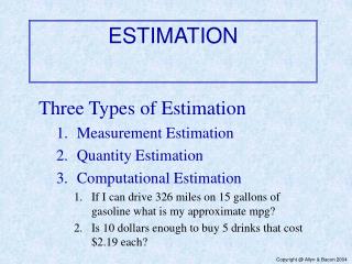
Estimation
Estimation. Statistics with Confidence. Estimation. Before we collect our sample, we know:.

Estimation
E N D
Presentation Transcript
Estimation Statistics with Confidence
Estimation Before we collect our sample, we know: Repeated sampling sample means would stack up in a normal curve, Centered on the true population mean, With a standard error (measure of dispersion) that depends on 1. population standard deviation 2. sample size -3z -2z -1z 0z 1z 2z 3z
Estimation But we do not know: 1. True Population Mean 2. Population Standard Deviation Repeated sampling sample means would stack up in a normal curve, Centered on the true population mean, With a standard error (measure of dispersion) that depends on 1. population standard deviation 2. sample size -3z -2z -1z 0z 1z 2z 3z
Estimation Will our sample be one of these (accurate)? Or one of these (inaccurate)? -3z -2z -1z 0z 1z 2z 3z
Estimation Which is more likely? accurate? or inaccurate? -3z -2z -1z 0z 1z 2z 3z 68% 95%
Estimation We’re most likely to get close to the true population mean… Our sample’s mean is the best guess of the population mean, but it is not precise. -3z -2z -1z 0z 1z 2z 3z 68% 95%
Estimation And if we increase our sample size (n)… -3z -2z -1z 0z 1z 2z 3z 68% 95%
Estimation And if we increase our sample size our sample mean is an even better estimate of the population mean, we are more precise! -3 -2 -1 0 1 2 3 -3z -2z -1z 0z 1z 2z 3z 68% 95%
Estimation We know that the standard deviation of this pile of samples (standard error) equals the population standard deviation () divided by the square root of the sample size (n). -3 -2 -1 0 1 2 3 68% 95%
Estimation But we do not know the population standard deviation! What is our best guess of that? -3 -2 -1 0 1 2 3 68% 95%
Estimation Our best guess of the population standard deviation is our sample’s s.d.! On average, this s.d. gives population . In fact, when we calculate that, we use “n – 1” to make our “estimate” larger to reflect that dispersion of a sample is smaller than a population’s. (Yi – Y)2 s = n - 1 = Cases in the sample 0 5 10 15 20 25 30 35 0 5 10 15 20 25 30 35 Population Dispersion Sample Dispersion
Estimation So now we know that we can use the sample standard deviation to stand in for the population’s standard deviation. So we can use the formula for standard error with that s estimate and get a good estimate s.e = of the dispersion of the n sampling distribution. -3 -2 -1 0 1 2 3 68% 95%
Estimation Now we know some limits on how far off our sample mean is likely to be from the true population mean! 68% of means will be within +/- 1 s.e. 95% of means will be within +/- 2 s.e. s s.e. = n -3 -2 -1 0 1 2 3 68% 95%
Estimation For example, if we took GPAs from a sample of 625 students and our s was .50… 68% of means would be within +/- 1*(.02) 95% of means would be within +/- 2*(.02) .5 s.e. = 625 = 0.02 -3 -2 -1 0 1 2 3 [0.02] 68% 95%
Estimation GPAs from a sample of 625 students with s = .50… If our sample were this one, our estimate of the mean would be correct! .5 s.e. = 625 = 0.02 -3 -2 -1 0 1 2 3 68% 95%
Estimation GPAs from a sample of 625 students with s = .50… But what if it were this one? We’d be slightly wrong, but well within +/- 2 *(.02) 95% of samples would be! .5 s.e. = 625 = 0.02 -3 -2 -1 0 1 2 3 68% 95%
Estimation A sample’s mean is the best estimate of the population mean. But what if we base our estimate on this erroneous sample? s s.e. = n -3 -2 -1 0 1 2 3 68% 95%
Estimation Let’s create a “measuring device” with our sampling distribution and center it over our sample’s mean. Check it Out! The true mean falls within the 95% bracket. s s.e. = n -3 -2 -1 0 1 2 3 68% 95%
Estimation What if the sample we collected were this one? …and we used the measuring device again? Check it Out! The true mean falls within the 95% bracket. s s.e. = n -3 -2 -1 0 1 2 3 68% 95%
Estimation The sampling distribution allows us to: 1. Be humble and admit that our sample statistic may not be the population’s and 2. Forms a measuring device with which we can determine a range where the true population mean is likely to fall... this is called a confidence interval.
Estimation If you calculate your sampling distribution’s standard error, you can form a device that tells you that if your sample mean is wrong, there is a documented a range in which the true population mean is likely 2Xist. Check it Out! The true mean falls within the 95% bracket. s s.e. = n Sample -3 -2 -1 0 1 2 3 68% 95%
Estimation For example, if we took GPAs from a sample of 625 students and our mean was 2.5 and s.d. was .50… We make a confidence interval (C.I.)by… Calculating the s.e. (.02) and Going +/- 2 * s.e. from the mean. .5 s.e. = 625 = 0.02 =2.52 -3 -2 -1 0 1 2 3 68% 95% 95% C.I. = 2.5 +/- 2(.02) = 2.46 to 2.54 We are 95% confident that the true mean is in this range!
Estimation Guys… This is power! Knowing that the spread of 95% of normally distributed sample means has outer limits… We know that if we put these limits around our sample mean… We have defined the range where the population mean has a 95% probability of being!
Estimation Our sample statistics provide enough information to give us a great estimation (highly educated guess) about population statistics. We do this without needing to know the population mean—without needing to have a census.
Estimation Another Example: Sample of 2,500 with an average income of $28,000 with a standard deviation of $8,000. Provide a 95% C.I. = M +/- 2 * (s.e.) • s.e. = $8,000/2,500 = $160 • 2 * $160 = $320 • C.I. = $28,000 +/- $320 C.I. >>> $27,680 to $28,320 s s.e. = n
Estimation Another Example: Sample of 2,500 with an average income of $28,000 with a standard deviation of $8,000. Provide a 95% C.I. = M +/- 2 * (s.e.) • s.e. = $8,000/2,500 = $160 • 2 * $160 = $320 • C.I. = $28,000 +/- $320 C.I. >>> $27,680 to $28,320 We are 95% confident that the true mean falls from $27,680 up to $28,320
Estimation NO WAIT! We’re wrong! Technically speaking, on a normal curve, 95% of cases fall between +/- 1.96 standard deviations rather than 2. (Check your book’s table.) Empirical Rule vs. Actuality 68% 1z 0.99z 95% 2z 1.96z 99.9973% 3z 3z
Estimation Another Example: Sample of 2,500 with an average income of $28,000 with a standard deviation of $8,000. Provide a 95% C.I. = M +/- 1.96 * (s.e.) • s.e. = $8,000/2,500 = $160 • 1.96 * $160 = $313.6 • C.I. = $28,000 +/- $313.6 C.I. >>> $27,686.4 to $28,313.6 We are 95% confident that the population mean falls between $27,686.4 and $28,313.6
Estimation Another Example: Sample of 2,500 with an average income of $28,000 with a standard deviation of $8,000. What if we want a 99% confidence interval, What z do we use? Check the table in your book!
Estimation Another Example: Sample of 2,500 with an average income of $28,000 with a standard deviation of $8,000. What if we want a 99% confidence interval? 99% fall between +/- 2.58 z’s
Estimation Another Example: Sample of 2,500 with an average income of $28,000 with a standard deviation of $8,000. What if we want a 99% confidence interval? • s.e. = $8,000/2,500 = $160 • 2.58 * $160 = $412.8 • C.I. = $28,000 +/- $412.8 CI >>> $27,587.2 to $28,412.8 We are 99% confident that the population mean falls between these values. Why did the interval get wider than 95% CI’s which was $27,686.4 to $28,313.6???
Estimation 99% CI >>> $27,587.2 to $28,412.8 Why did the interval get wider than 95% CI’s which was $27,686.4 to $28,313.6??? M -3 -2 -1 0 1 2 3 68% 99% 95%
Estimation … Let’s recap: We can say that 95% of the sample means in repeated sampling will always be in the range marked by -1.96 over to +1.96 standard errors. Self-esteem 15 20 25 30 35 40 1.96 Z-3 -2 -1 0 1 2 3 -1.96 95% Range z -3 -2 -1 0 1 2 3
Estimation And remember: If we don’t know the true population mean, 95% of the time a 95% confidence interval would contain the true population mean! Self-esteem 15 20 25 30 35 40 95% Ranges for different samples.
Estimation If we want that range to contain the true population mean 99% of the time (99% confidence interval) we just construct a wider interval, corresponding with 2.58 z’s. Self-esteem 15 20 25 30 35 40 99% Ranges for different samples, overlaying 95% intervals.
Estimation 1.96z The sampling distribution’s standard error is a measuring stick that we can use to indicate the range of a specified middle percentage of sample means in repeated sampling. 95% 1z 68% 3z 99.99% 25 -3 -1.96 -1 0 1 1.96 3 68% 95% 99.99%
Estimation Another Confidence Interval Example: I collected a sample of 2,500 with an average self-esteem score of 28 with a standard deviation of 8. What if we want a 99% confidence interval? CI = Mean +/- z * s.e. • Find the standard error of the sampling distribution: s.d. / n = 8/50 = 0.16 • Build the width of the Interval. 99% corresponds with a z of 2.58. 2.58 * 0.16 = 0.41 • Insert the mean to build the interval: 99% C.I. = 28 +/- 0.41 The interval: 27.59 to 28.41 We are 99% confident that the population mean falls between these values.
Estimation And if we wanted a 95% Confidence Interval instead? I collected a sample of 2,500 with an average self-esteem score of 28 with a standard deviation of 8. What if we want a 99% confidence interval? CI = Mean +/- z * s.e. • Find the standard error of the sampling distribution: s.d. / n = 8/50 = 0.16 • Build the width of the Interval. 99% corresponds with a z of 2.58. 2.58 * 0.16 = 0.41 • Insert the mean to build the interval: 99% C.I. = 28 +/- 0.41 The interval: 27.59 to 28.41 We are 99% confident that the population mean falls between these values. 95% X 95% 1.96 X X X X 0.31 1.96 X X 95% 0.31 X X 27.69 to 28.31 X 95%
Estimation By centering my sampling distribution’s +/- 1.96z range around my sample’s mean... • I can identify a range that, if my sample is one of the middle 95%, would contain the population’s mean. Or • I have a 95% chance that the population’s mean is somewhere in that range.
Estimation By centering my sampling distribution’s +/- 1.96z range around my sample’s mean... • I can identify a range that, if my sample is one of the middle 95%, would contain the population’s mean. Or • I have a 95% chance that the population’s mean is somewhere in that range. X 2.58z X 99% 99% X