Market Efficiency and Equilibrium Analysis on Taxes and Subsidies
Understand the impact of taxes, subsidies, and market interventions on economic efficiency and equilibrium through real-world examples. Learn about consumer surplus, producer surplus, deadweight loss, and more.

Market Efficiency and Equilibrium Analysis on Taxes and Subsidies
E N D
Presentation Transcript
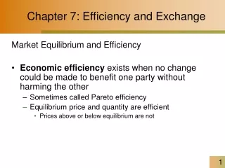
Chapter 7: Efficiency and Exchange Market Equilibrium and Efficiency • Economic efficiency exists when no change could be made to benefit one party without harming the other • Sometimes called Pareto efficiency • Equilibrium price and quantity are efficient • Prices above or below equilibrium are not
Price Below Equilibrium • Suppose milk is $1 per gallon S 2.50 2.00 1.50 Price ($/gallon) 1.00 0.50 D 1 2 3 4 5 Quantity (1,000s of gallons/day)
Price Below Equilibrium • A buyer offers $1.25 per gallon S 2.50 2.00 1.50 Price ($/gallon) 1.25 1.00 0.50 D 1 2 3 4 5 Quantity (1,000s of gallons/day)
Price above Equilibrium S 2.50 2.00 1.75 Only equilibrium price is efficient 1.50 Price ($/gallon) 1.00 0.50 D 1 2 3 4 5 Quantity (1,000s of gallons/day)
Heating Oil Market 2.00 S 1.80 1.60 Consumer surplus = $900/day 1.40 Producer surplus = $900/day 1.20 Price ($/gallon) 1.00 .80 D 1 2 3 4 5 8 Quantity (1,000s of gallons/day)
Price Ceiling on Heating Oil Consumer surplus = $900/ day 2.00 1.80 S 1.60 Lost surplus = $800/ day 1.40 1.20 Price ($/gallon) 1.00 Producer surplus = $100/ day 0.80 D 1 2 3 4 5 8 Quantity (1,000s of gallons/day)
Price Subsidies for Bread Price ($/loaf) $4.00 Consumer Surplus = $4 M/month $3.00 S $2.00 Consumer Surplus = $9 M/month $1.00 S with subsidy D 2 4 6 8 Quantity (millions of loaves/month) BUT…
The Cost of the Subsidy • BUT … • The government loses $1 on every loaf • Imports 6 million loaves for $2 per loaf • Government losses are $6 million • The net benefit of the subsidy program • Consumer surplus – government losses • Net benefit = $3 million
Taxes on Sellers • Tax program • Seller reports sales in units to government • Seller pays a fixed dollar amount per unit sold • A tax on the seller shifts the supply curve up by the amount of the tax • Vertical interpretation of the supply curve • For each level of output, seller charges his marginal cost PLUS the tax
Tax on Avocado Sellers S + tax S 6 5 4 3.50 Price ($/pound) 3 2.50 2 1 D 1 2 3 4 5 2.5 Quantity (millions of pounds/month)
Taxes and Perfectly Elastic Supply Price ($/car) If supply is perfectly elastic, buyers pay all of the tax S + $100 $20,100 S $20,000 D 1.9 2.0 Quantity (millions of cars/month)
Tax on Avocado Sellers • Before Tax • Consumer surplus = $4.5 M • Producer surplus = $4.5 M P S 6 3 P S + tax D 6 3 Q 3.50 • After Tax • Consumer surplus = $3.125 M • Producer surplus = $3.125 M • Total surplus = $6.25 M • Loss = $2.75 M 1 D Q 2.5
Taxes and Price Elasticity of Demand More Elastic Demand Less Elastic Demand P P S + T S + T 2.60 2.40 S S 2.00 2.00 1.60 1.40 D1 D2 19 24 21 24 Q Q Consumers pay a smaller share of the tax when demand is more elastic
Taxes and Deadweight Loss More Elastic Demand Less Elastic Demand P P Deadweight loss Deadweight loss S + T S + T 2.60 2.40 S S 2.00 2.00 1.60 1.40 D1 D2 19 24 21 24 Q Q Deadweight loss is larger when demand is relatively elastic