Download

1 / 42
430 likes | 636 Vues
The “Second Law” of Probability: Entropy Growth in the Central Limit Theorem. Keith Ball. The second law of thermodynamics. Joule and Carnot studied ways to improve the efficiency of steam engines.

E N D
The “Second Law” of Probability: Entropy Growth in the Central Limit Theorem. Keith Ball
The second law of thermodynamics Joule and Carnot studied ways to improve the efficiency of steam engines. Is it possible for a thermodynamic system to move from state A to state B without any net energy being put into the system from outside? A single experimental quantity, dubbed entropy, made it possible to decide the direction of thermodynamic changes.
The second law of thermodynamics The entropy of a closed system increases with time. The second law applies to all changes: not just thermodynamic. Entropy measures the extent to which energy is dispersed: so the second law states that energy tends to disperse.
The second law of thermodynamics Maxwell and Boltzmann developed a statistical model of thermodynamics in which the entropy appeared as a measure of “uncertainty”. Uncertainty should be interpreted as “uniformity” or “lack of differentiation”.
The second law of thermodynamics Closed systems become progressively more featureless. We expect that a closed system will approach an equilibrium with maximum entropy.
Information theory Shannon showed that a noisy channel can communicate information with almost perfect accuracy, up to a fixed rate: the capacity of the channel. The (Shannon) entropy of a probability distribution: if the possible states have probabilities then the entropy is Entropy measures the number of (YES/NO) questions that you expect to have to ask in order to find out which state has occurred.
Information theory You can distinguish 2k states with k (YES/NO) questions. If the states are equally likely, then this is the best you can do. It costs k questions to identify a state from among 2k equally likely states.
Information theory It costs k questions to identify a state from among 2k equally likely states. It costs log2 n questions to identify a state from among n equally likely states: to identify a state with probability 1/n.
The entropy Entropy = p1log2(1/p1) + p2 log2 (1/p2) + p3 log2 (1/p3) + …
Continuous random variables For a random variable X with density f the entropy is The entropy behaves nicely under several natural processes: for example, the evolution governed by the heat equation.
If the density f measures the distribution of heat in an infinite metal bar, then f evolves according to the heat equation: The entropy increases: Fisher information
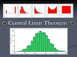
The central limit theorem If Xi are independent copies of a random variable with mean 0 and finite variance, then the normalized sums converge to a Gaussian (normal) with the same variance. Most proofs give little intuition as to why.
The central limit theorem Among random variables with a given variance, the Gaussian has largest entropy. Theorem (Shannon-Stam) If X and Y are independent and identically distributed, then the normalized sum has entropy at least that of X and Y.
Idea The central limit theorem is analogous to the second law of thermodynamics: the normalized sums have increasing entropy which drives them to an “equilibrium” which has maximum entropy.
The central limit theorem Linnik (1959) gave an information-theoretic proof of the central limit theorem using entropy. He showed that for appropriately smoothed random variables, if Sn remains far from Gaussian, then Sn+1 has larger entropy than Sn. This gives convergence in entropy for the smoothed random variables but does not show that entropy increases with n.
Problem: (folklore or Lieb (1978)). Is it true that Ent(Sn) increases with n? Shannon-Stam shows that it increases as n goes from 1 to 2 (hence 2 to 4 and so on). Carlen and Soffer found uniform estimates for entropy jump from 1 to 2. It wasn’t known that entropy increases from 2 to 3. The difficulty is that you can't express the sum of 3 independent random variables in terms of the sum of 2: you can't add 3/2 independent copies of X.
The Fourier transform? The simplest proof (conceptually) of the central limit theorem uses the FT. If X has density f whose FT is then the FT of the density of is . The problem is that the entropy cannot easily be expressed in terms of the FT. So we must stay in real space instead of Fourier space.
Example: Suppose X is uniformly distributed on the interval between 0 and 1. Its density is: When we add two copies the density is:
For 9 copies the density is a spline defined by 9 different polynomials on different parts of the range. The central polynomial (for example) is: and its logarithm is?
The second law of probability A new variational approach to entropygives quantitative measures of entropy growth and proves the “second law”. Theorem (Artstein, Ball, Barthe, Naor) If Xi are independent copies of a random variable with finite variance, then the normalized sums have increasing entropy.
Starting point: used by many authors. Instead of considering entropy directly, we study the Fisher information: Among random variables with variance 1, the Gaussian has the smallest Fisher information, namely 1. The Fisher information should decrease as a process evolves.
The connection (we want) between entropy and Fisher information is provided by the Ornstein-Uhlenbeck process (de Bruijn, Bakry and Emery, Barron). Recall that if the density of X(t) evolves according to the heat equation then The heat equation can be solved by running a Brownian motion from the initial distribution. The Ornstein-Uhlenbeck process is like Brownian motion but run in a potential which keeps the variance constant.
The Ornstein-Uhlenbeck process A discrete analogue: You have n sites, each of which can be ON or OFF. At each time, pick a site (uniformly) at random and switch it. X(t)= (number on)-(number off).
The Ornstein-Uhlenbeck process A typical path of the process.
The Ornstein-Uhlenbeck evolution The density evolves according to the modified diffusion equation: From this: As the evolutes approach the Gaussian of the same variance.
The entropy gap can be found by integrating the information gap along the evolution. In order to prove entropy increase, it suffices to prove that the information decreases with n. It was known (Blachman-Stam) that .
Main new tool:a variational description of the information of a marginal density. If w is a density on and e is a unit vector, then the marginal in direction e has density
Main new tool: The density h is a marginal of w and The integrand is non-negative if h has concave logarithm. Densities with concave logarithm have been widely studied in high-dimensional geometry, because they naturally generalize convex solids.
The Brunn-Minkowski inequality x Let A(x) be the cross-sectional area of a convex body at position x. Then log A is concave. The function A is a marginal of the body.
The Brunn-Minkowski inequality x We can replace the body by a function with concave logarithm. If w has concave logarithm, then so does each of its marginals. If the density h is a marginal of w, the inequality tells us something about in terms of
The Brunn-Minkowski inequality If the density h is a marginal of w, the inequality tells us something about in terms of We rewrite a proof of the Brunn-Minkowski inequality so as to provide an explicit relationship between the two. The expression involving the Hessian is a quadratic form whose minimum is the information of h. This gives rise to the variational principle.
The variational principle TheoremIf w is a density and e a unit vector then the information of the marginal in the direction e is where the minimum is taken over vector fields p satisfying
Technically we have gained because h(t) is an integral: not good in the denominator. The real point is that we get to choose p. Instead of choosing the optimal p which yields the intractable formula for information, we choose a non-optimal p with which we can work.
Proof of the variational principle. so If p satisfies at each point, then we can realise the derivative as since the part of the divergence perpendicular to e integrates to 0 by the Gauss-Green (divergence) theorem.
Hence There is equality if This divergence equation has many solutions: for example we might try the electrostatic field solution. But this does not decay fast enough at infinity to make the divergence theorem valid.
The right solution for p is a flow in the direction of e which transports between the probability measures induced by w on hyperplanes perpendicular to e. For example, if w is 1 on a triangle and 0 elsewhere, the flow is as shown. (The flow is irrelevant where w = 0.) e
How do we use it? If w(x1,x2,…xn) = f(x1)f(x2)…f(xn), then the density of is the marginal of w in the direction (1,1,…1). The density of the (n-1)-fold sum is the marginal in direction (0,1,…,1) or (1,0,1,…,1) or…. Thus, we can extract both sums as marginals of the same density. This deals with the “difficulty”.
Proof of the second law. Choose an(n-1)-dimensional vector field p with and . In n-dimensional space, put a “copy” of p on each set of n-1 coordinates. Add them up to get a vector field with which to estimate the information of the n-fold sum.
As we cycle the “gap” we also cycle the coordinates of p and the coordinates upon which it depends: Add these functions and normalise:
We use P to estimate J(n). The problem reduces to showing that if then The trivial estimate (using ) gives n instead of n-1. We can improve it because the have special properties. There is a small amount of orthogonality between them because is independent of the i coordinate.
The second law of probability Theorem If Xi are independent copies of a random variable with variance, then the normalized sums have increasing entropy.