Download
1 / 37
380 likes | 541 Vues
Continuous Probability Distributions And The Central Limit Theorem. Continuous Distributions.

E N D
Continuous Probability Distributions And The Central Limit Theorem
Continuous Distributions In all of the previous examples that we have studied so far, we have been dealing with samples taken from a discrete set of population values – the possible values of the parameter of interest were limited to a finite set of possibilities. • For example: • The ages measured in years of Oscar-winning actors • The heights measured to the nearest inch of players in the NBA • The temperatures measured to the nearest degree of days in 2009 • The grades expressed in integers on an exam • The weights expressed to the nearest tenth of a gram of dimes In a discrete distribution every value in the set of possible outcomes has a finite chance of occurring
0 1 2 3 4 5 ContinuousDistributions Uniform Distribution Suppose we discount our inability to measure beyond a certain precision and assume that all values of x in the range 1 x 5 are possible outcomes for a measurement x. If we assume that the measurement is equally likely to be anywhere in this range, we depict the distribution as follows: f(x) x
0 1 2 3 4 5 Continuous Distributions f(x) is called the probability density associated with the point x. Since there are an infinite number of real values in the line segment from 1 to 5, we cannot assign a non-zero probability to any one value being selected. It only makes sense to talk about the probability of x lying in a range between two values x1 and x2 x1 x2 f(x) x
0 1 2 3 4 5 Continuous Distributions Step 1: Normalize the area in the distribution (inside the rectangle) to 1 Area = f(x) * (5 – 1) = 1 then f(x) = ¼ for all 1 x 5 Step 2: Find the area between x1 = 2 and x2 = 3 P(2 x 3) = f(x) * (x2 – x1) = ¼ * 1 = ¼ x1 x2 f(x) x
0 1 2 3 4 5 Continuous Distributions In a continuous distribution • f(x) represents a probability density associated with a value x • The area under the curve f(x) is normalized to 1 • The probability that a selected value of x lies in the region Δx = x2 – x1 is given by the formula P(x1 x x2) = f(x) * Δx x1 x2 f(x) x
Continuous Distributions What do we mean by a probability density? • The probability density f(x) is the probability/linear length • The variable x may represent a value whose units are distance, time, weight, or some other measure like parts per hundred • The horizontal axis over which x is measured is marked out in gradations of the units of variable x. (for example– if x represents weights of people in a population, the x-axis will be marked out in gradations of pounds or kilograms • For the uniform distribution, f(x) is a constant over the entire range of x, but in general, the probability density may vary over that range. • For a continuous distribution we can only find the probability that a selected value of x will lie in a range Δxbetween two other points. • P(x1 x x2) = the area under the curve f(x) * Δx • The probability that x is exactly equal to a single value x1, is 0. • A single point is a linear length of measure 0, and our formula: • P(x1 x x2) = the area under the curve f(x) * Δx = 0, since Δx = 0
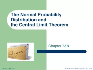
Continuous Distributions The Normal Distribution The most important example of a continuous distribution is the normal distribution. The normal distribution is: • Bell shaped • Symmetrical • Unimodal • Unbounded • Has the property that the mean, median and mode are all equal
f(x) x Symmetric Unbounded Mean = Median = Mode Continuous Distributions Bell-shaped
f(x) -3σ 3σ -1σ 1σ -2σ 2σ x 99.7% of the values lie within ±3σ of the mean About 95% of the values lie within ±2σ of the mean Continuous Distributions μ 68% of the values are within ± 1σ of the mean
f(x) x Continuous Distributions μ To convert a normal distribution with a mean of μ and standard deviation into a standard normal distribution with mean 0, standard deviation 1, we convert all of the x-scores into corresponding z-scores using the formula z = (x - )/
f(x) x Continuous Distributions μ x1 x2 Let us suppose that we have a normally distributed population with a mean of 20 and a standard deviation of 5 and we want to find the probability that a selected member of this population lies in the range of x1 = 21 to x2 = 24.5 represented by the shaded area in the above diagram
Continuous Distributions Step 1: Convert the problem of finding the probability of selecting a value in the interval between x1 and x2 in this normal distribution into the probability of finding a value in the corresponding interval in the standard normal distribution z2 = (24.5 – 20) / 5 = 0.900 z1 = (21 – 20) / 5 = 0.200 f(z) 0 z1 z2 z
Find z2 = 0.90 (table reads to nearest hundredths) Continuous Distributions Step 2: Use the Standard Normal Distribution Table on the back cover to find the probability that a selected value of z lies in the shaded region (same as the area under the curve inside the shaded region of the previous diagram) .00 .01 .02 ….. .. .09 0.0 0.1 0.2 …. … 0.9 1.0 … 0.5000 0.5040 0.5080 0.5359 0.5398 0.5438 0.5478 0.5753 0.5793 0.5832 0.5871 0.6141 0.8159 0.8186 0.8212 0.8389 0.8413 Find z1 = 0.20 (table reads to nearest hundredths)
Continuous Distributions The area to the left of z1 (shaded blue) is = 0.5793 from the table The area to the left of z2 (shaded red) is = 0.8159 from the table The area in the interval between z1 and z2 (only shaded red) = 0.8159 – 0.5793 f(z) z 0 z1 z2 P(21 x 24.5) = P(0.20 z 0.90) = 0.8159 – 0.5793 = 0.2366
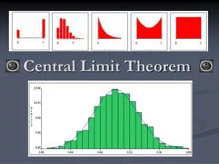
The Central Limit Theorem
P(x) ¼ 0 1 2 3 4 The Central Limit Theorem Consider a population consisting ofthe numbers 1, 2, 3, 4, Assume there are an essentially infinite number of each digit in the population (sampling without replacement does not affect the proportion of each value) and that ¼ of the values correspond to each digit. The population is depicted below: This distribution is clearly discrete (only 4 possible values), but we will use it to indicate properties of the continuous sampling distribution
The Central Limit Theorem First, calculate the population mean and standard deviation of this population distribution. = iP(xi) xi = ¼ (1) + ¼ (2) + ¼ (3) + ¼ ( 4) = 2.5 2 = iP(xi) (xi - )2 = ¼ ((1 – 2.5)2 + (2 – 2.5)2 + (3 – 2.5)2 + (4 – 2.5)2 ) = ¼ (2.25 + 0.25 + 0.25 + 2.25) = 1.25 = 1.25 = 1. 118
The Central Limit Theorem Now, let’s look at all possible samples of size 3 from this population Let x’ = the sample mean (1,1,1) x’ = 1 (1,1,2), (1,2,1), (2,1,1) x’ = 1.33 (1,1,3), (1,3,1), (3,1,1) x’ = 1.67 (1,1,4), (1,4,1), (4,1,1) x’ = 2 (1,2,2), (2,1,2), (2,2,1) x’ = 1.67 (1,3,3), (3,1,3), (3,3,1) x’ = 2.33 (1,4,4), (4,1,4), (4,4,1) x’ = 3 (1,2,3), (1,3,2), (2,1,3) (2,3,1), (3,1,2), (3,2,1) x’ = 2 (1,2,4), (1,4,2), (2,1,4) (2,4,1), (4,1,2), (4,2,1) x’ = 2.33 (1,3,4), (1,4,3), (3,1,4) (3,4,1), (4,1,3), (4,3,1) x’ = 2.67 (2,2,2) x’ = 2 (2,3,4), (2,4,3), (3,2,4) (3,4,2), (4,2,3), (4,3,2) x’ = 3 (2,2,3), (2,3,2), (3,2,2) x’ = 2.33 (2,2,4), (2,4,2), (4,2,2) x’ = 2.67 (2,3,3), (3,2,3), (3,3,2) x’ = 2.67 (2,4,4), (4,2,4), (4,4,2) x’ = 3.33 (3,3,3) x’ = 3 (3,3,4), (3,4,3), (4,3,3) x’ = 3.33 (4,4,3), (4,3,4), (3,4,4) x’ = 3.67 (4,4,4) x’ = 4
The Central Limit Theorem On the previous page we listed all 64 possible samples that could be selected from our original (discrete) distribution. We now examine the distribution of sample means Sample mean(x’) number of occurrences – f(x’) 1.00 1 1.33 3 1.67 6 2.00 10 2.33 12 2.67 12 3.00 10 3.33 6 3.67 3 4.00 1 64
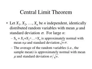
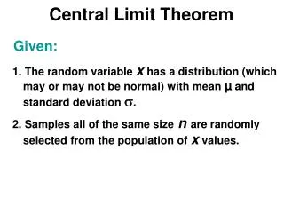
The Central Limit Theorem • Given: We are selecting samples of size n from a population (that may or may not be normal) with a population mean and a population standard deviation • Result: • 1. The distribution of sample means, x’, will, as the sample size n increases, approach a normal distribution. • The mean of all possible sample means for samples of size n will be the same as the population mean . • The standard deviation of all sample means is /n The Central Limit Theorem does not strictly apply to samples of size < 30 selected from a non-Normal population, but the small sample size (3) for our example allows us to enumerate all possible samples from the original population and will give approximate agreement to result # 1 above, and exact agreement with results # 2 and # 3.
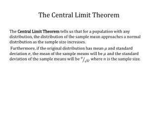
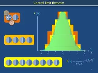
f(x) x 0 1.0 2.0 3.0 4.0 symmetric Semi-bell shaped bounded The Central Limit Theorem Let’s plot the frequency of occurrence of each of the values for the sample means 12 10 8 6 4 2 The distribution is: discrete
The Central Limit Theorem Now let’s calculate the (population) mean and standard deviation for the distribution of sample means of size n = 3. x’ =(x’f(x’) x’)/N = (1 1 + 3 1.33 + 6 1.67 + 10 2 + 12 2.33 + 12 2.67 + 10 3 + 6 3.33 + 3 3.67 + 1 4)/64 = 160/64 = 2.5 x’2 = (x’f(x’)/n (x’)2 – x’2) = (1 + 3 1.332 + 6 1.672 + 10 22 + 12 2.332 + 12 2.672 + 10 32 + 6 3.332 + 3 3.672 + 42)/64 – 2.52 = 6.667 – 6.250 = 0.4167 x’ = 0.4167 = 0.6455
The Central Limit Theorem The Central Limit Theorem stipulates that x’ = (the mean of the sampling distribution = the mean of the population from which the samples are drawn) and x’ = / n In our example, we have found that Mean of sampling distribution x’ = 2.5 Mean of population = 2.5 Standard Deviation of sampling dist. x’ = 0.6455 /n = 1.118 /3 = 0.6455
x’ f(x) -1 +1 -2 +2 x 0 1.0 2.0 3.0 4.0 62/64 = 96.88% of values lie within 2 The Central Limit Theorem The distribution of sample means -- x’= 2.5, x’ = 0.645 12 10 8 6 4 2 44/64 = 68.75% of values lie within of mean
The Central Limit Theorem The previous example serves to illustrate the Central Limit Theorem The sample size of n = 3 was chosen so that ALL of the samples in the sampling distribution could be enumerated and the population of sample means for sample size n = 3 could be plotted and its parameters calculated. The sample size n = 3 was too small to produce an approximately normal distribution or quasi-continuous distribution, BUT • Even for small samples from an original population that was not normal • The distribution of sample means is symmetric and somewhat bell-shaped • The mean of the sampling distribution equals the mean of the original population • The standard deviation of the sampling distribution equals the standard deviation of the original population divided by the square root of the sample size • The fraction of the values in the sampling distribution that are within 1 and 2 standard deviations from the mean are in substantial agreement with those fractions in a normal distribution
Central Limit Theorem Suppose we change (skew) the original population such that we have the following probabilities: x = 1 p(x) = 0.125 (1/8) x = 2 p(x) = 0.125 (1/8) x = 3 p(x) = 0.250 (1/4) x = 4 p(x) = 0.500 (1/2) = 0.125 * 1 + 0.125 * 2 + 0.25 * 3 + 0.5 * 4 = 3.125 2 = 0.125 * (1 – 3.125)2 + 0.125 * (2 – 3.125)2 + 0.25 * (3 – 3.125)2 + 0.5 * (4 – 3.125)2 = 1.109375 = 1.109375 = 1.0533
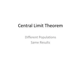
= 3.125 P(x) ½ -1 1 ¼ x 0 1 2 3 4 Central Limit Theorem Population mean = 3.125 Population standard deviation = 1.0533
Central Limit Theorem The same 64 samples that can be selected from this population now produce sample means with the probabilities tabulated below: Sample mean(x’) (x’)2 p(x’) x’ * p(x) (x’)2 * p(x’) 1.00 1.0000 .00195 .00195 .00195 1.33 1.7778 .00586 .00781 .01042 1.67 2.7778 .01758 .02930 .04883 2.00 4.0000 .04883 .09765 .19530 2.33 5.4444 .08203 .19113 .44662 2.67 7.1111 .14063 .37498 .99995 3.00 9.0000 .20313 .60937 1.88280 3.33 11.1111 .18750 .62500 2.08333 3.67 13.4444 .18750 .68750 2.52080 4.00 16.0000 .12500 .500002.00000 3.12464 10.18948 x’ = 3.124 2 = 10.18948 – (3.12464)2 = 0.426103 = 0.6527
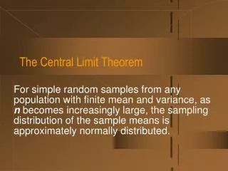
x’ = 3.124 p(x) -1 +1 0.20 0.15 0.10 0.05 0.00 x 0 1.0 2.0 3.0 4.0 Central Limit Theorem Now graph the distribution of the sample means
Central Limit Theorem When the initial population is not symmetric, the distribution of sample means selected from the original population does not produce as good an agreement with the results of the central limit theorem for samplesof small size. From the previous graph we see that the distribution of sample means is not symmetric or bell-shaped. Population parameters: = 3.125 = 1.0533 Distribution of sample means with n = 3: x’ = 3.124 x’ = .6527 x’ = .6527 not a good fit for /n = 1.0533/ 3 = .608
The Binomial Distribution • Let: • n = number of trials • p = probability of a success on any one trial • q = probability of failure on any one trial • The outcome of each trial is independent of the outcome on preceding trials • x = the number of successes in n trials Then the probability of exactly x successes in n trials is given by the term nCx pxqn-x in the expansion of the binomial (p + q)n The value of this term for a given (n, x, p) can be read from the Binomial Probability Tables in the text.
The Binomial Distribution Example: In 1941, Ted Williams was batting .39997(which rounded up to .400) on the last day of the season. He was given the choice not to play in the doubleheader scheduled for that day and preserve his 400 average, but decided to play anyway and got 6 hits in 8 (official) at bats to finish the year hitting 406. What was the probability that Ted would go 6 for 8 on that date? What was the probability that he would end up hitting 400 if he were to get 8 official at bats on that day? Assume the outcome of each at bat was independent of any other n = 8 number of trials x = 6 number of successes (hits) p = 0.40 probability of a hit in any at bat q = 1 – p = 0.60 probability of an out in each at bat
p n x .01 .05 .10 .20 .30 .40 .50 To end the day batting over 400, Ted will need to get 4 or more hits in his 8 at bats P(4 or more hits) = .232 + .124 + .041 + .008 + .001 = 0.406 The Binomial Distribution From the Binomial Probability Tables we have the following: ……….. 8 0 1 2 3 4 5 6 7 8 Probability of exactly 6 hits in 8 AB = 0.041 ………………………………………………………………………… 0+ 0+ .005.046 .136 .232 .273 0+ 0+ 0+ .009 .047 .124 .219 0+ 0+ 0+ .001 .010 .041 .109 0+ 0+ 0+ 0+ .001 .008 .031 0+ 0+ 0+ 0+ 0+ .001 .004
The Normal Approximation of the Binomial Distribution The discrete Binomial Distribution may be approximated using the continuous Normal Distribution if the following are true: • np 5, and • nq 5 Then the binomial distribution may be approximated by a normal distribution with mean = np and standard deviation = npq
The Normal Approximation of the Binomial Distribution Example: Passenger Load on a Boeing 767-300 The aircraft has a seating capacity of 213 seats. When fully loaded, with passengers, crew, cargo, and fuel, the pilot must verify that the gross weight is below the maximum allowable limit, and the weight must be properly distributed so that balance of the aircraft is within safe acceptable limits. Instead of weighing the passengers, their weights are estimated according to FAA rules. Men have a mean weight of 172 pounds Women have a mean weight of 143 pounds Assume that if there are122 or more male passengers in the 213 seats, the load may have to be adjusted. Assume also that the probability of a man or woman booking a seat is 0.5. What is the probability of having 122 or more male passengers if the plane is fully booked? Step 1: np = nq = (213)(0.5) = 106.5 > 5 Normal approximation applies
The Normal Approximation of the Binomial Distribution Step 2: Find the mean and standard deviation of the approximate normal distribution • = np = 106.5 = npq = (213)(0.5)(0.5) = 7.297 Step 3: Represent the discrete value 122 by the interval (121.5,122.5) Step 4: Find probability that x 121.5 in this distribution Convert 121.5 to a z-score z = (x - )/ = (121.5 – 106.5)/7.297 = 2.06 Step 5: From the Standard Normal Table P(z 2.06) = 1 – 0.9803 = 0.0197