THE CENTRAL LIMIT THEOREM
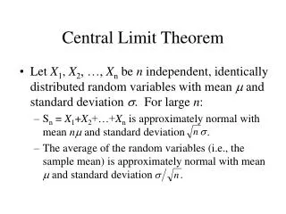
THE CENTRAL LIMIT THEOREM. The World is Normal Theorem. Sampling Distribution of x- normally distributed population. n=10. Sampling distribution of x: N ( , /10). /10. Population distribution: N( , ). . Normal Populations. Important Fact:


THE CENTRAL LIMIT THEOREM
E N D
Presentation Transcript
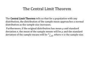
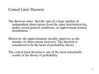
THE CENTRAL LIMIT THEOREM The World is Normal Theorem
Sampling Distribution of x- normally distributed population n=10 Sampling distribution of x: N( , /10) /10 Population distribution: N( , )
Normal Populations • Important Fact: • If the population is normally distributed, then the sampling distribution of x is normally distributed for any sample size n. • Previous slide
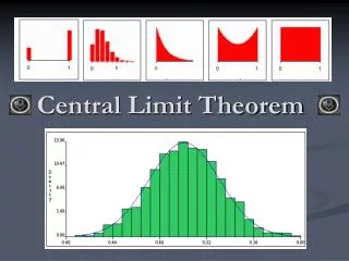
Population: interarrival times between consecutive customers at an ATM f(x) 0 time Non-normal Populations • What can we say about the shape of the sampling distribution of x when the population from which the sample is selected is not normal?
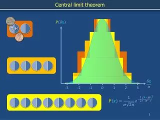
The Central Limit Theorem(for the sample mean x) • If a random sample of n observations is selected from a population (any population), then when n is sufficiently large, the sampling distribution of x will be approximately normal. (The larger the sample size, the better will be the normal approximation to the sampling distribution of x.)
The Importance of the Central Limit Theorem • When we select simple random samples of size n, the sample means we find will vary from sample to sample. We can model the distribution of these sample means with a probability model that is
How Large Should n Be? • For the purpose of applying the central limit theorem, we will consider a sample size to be large when n > 30.
Summary Population: mean ; stand dev. ; shape of population dist. is unknown; value of is unknown; select random sample of size n; Sampling distribution of x: mean ; stand. dev. /n; always true! By the Central Limit Theorem: the shape of the sampling distribution is approx normal, that is x ~ N(, /n)
The Central Limit Theorem(for the sample proportion p) • If a random sample of n observations is selected from a population (any population), and x “successes” are observed, then when n is sufficiently large, the sampling distribution of the sample proportion p will be approximately a normal distribution.
The Importance of the Central Limit Theorem • When we select simple random samples of size n, the sample proportions p that we obtain will vary from sample to sample. We can model the distribution of these sample proportions with a probability model that is
How Large Should n Be? • For the purpose of applying the central limit theorem, we will consider a sample size to be large when np > 10 and nq > 10
Population Parameters and Sample Statistics • The value of a population parameter is a fixed number, it is NOT random; its value is not known. • The value of a sample statistic is calculated from sample data • The value of a sample statistic will vary from sample to sample (sampling distributions)
Graphically n=64 Sampling distribution of x: N( , /n) = N(15, 4/8) x=4/64 = 4/8 Population distribution: = 15, = 4 = 4 = 15
Example 2 • The probability distribution of 6-month incomes of account executives has mean $20,000 and standard deviation $5,000. • a) A single executive’s income is $20,000. Can it be said that this executive’s income exceeds 50% of all account executive incomes? ANSWER No. P(X<$20,000)=? No information given about distribution of X
Example 2(cont.) • b) n=64 account executives are randomly selected. What is the probability that the sample mean exceeds $20,500?
Example 3 • A sample of size n=16 is drawn from a normally distributed population with mean E(x)=20 and SD(x)=8.
Example 3 (cont.) • c. Do we need the Central Limit Theorem to solve part a or part b? • NO. We are given that the population is normal, so the sampling distribution of the mean will also be normal for any sample size n. The CLT is not needed.
Example 4 • Battery life X~N(20, 10). Guarantee: avg. battery life in a case of 24 exceeds 16 hrs. Find the probability that a randomly selected case meets the guarantee.
Example 5 Cans of salmon are supposed to have a net weight of 6 oz. The canner says that the net weight is a random variable with mean =6.05 oz. and stand. dev. =.18 oz. Suppose you take a random sample of 36 cans and calculate the sample mean weight to be 5.97 oz. • Find the probability that the mean weight of the sample is less than or equal to 5.97 oz.
Population X: amount of salmon in a canE(x)=6.05 oz, SD(x) = .18 oz • X sampling dist: E(x)=6.05 SD(x)=.18/6=.03 • By the CLT, X sampling dist is approx. normal • P(X 5.97) = P(z [5.97-6.05]/.03) =P(z -.08/.03)=P(z -2.67)= .0038 • How could you use this answer?
Suppose you work for a “consumer watchdog” group • If you sampled the weights of 36 cans and obtained a sample mean x 5.97 oz., what would you think? • Since P( x 5.97) = .0038, either • you observed a “rare” event (recall: 5.97 oz is 2.67 stand. dev. below the mean) and the mean fill E(x) is in fact 6.05 oz. (the value claimed by the canner) • the true mean fill is less than 6.05 oz., (the canner is lying ).
Example 6 • X: weekly income. E(x)=600, SD(x) = 100 • n=25; X sampling dist: E(x)=600 SD(x)=100/5=20 • P(X 550)=P(z [550-600]/20) =P(z -50/20)=P(z -2.50) = .0062 Suspicious of claim that average is $600; evidence is that average income is less.
Example 7 • 12% of students at NCSU are left-handed. What is the probability that in a sample of 50 students, the sample proportion that are left-handed is less than 11%?