Central Limit Theorem

1. Central Limit Theorem Given: 1. The random variable x has a distribution (which may or may not be normal) with mean µ and standard deviation . 2. Samples all of the same size n are randomly selected from the population of xvalues.

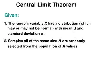
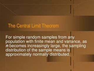
2. Central Limit Theorem Conclusions: 1. The distribution of sample x will, as the sample size increases, approach a normal distribution. 2. The mean of the sample means will be the population mean µ. 3. The standard deviation of the sample means will approach  n

3. Practical Rules Commonly Used: 1. For samples of size n larger than 30, the distribution of the sample means can be approximated reasonably well by a normal distribution. The approximation gets better as the sample size n becomes larger. 2. If the original population is itself normally distributed, then the sample means will be normally distributed for any sample sizen (not just the values of n larger than 30).

4. Notation the mean of the sample means  µx=µ

5. Notation the mean of the sample means the standard deviation of sample mean  µx=µ  x= n

6. Notation the mean of the sample means the standard deviation of sample mean  (often called standard error of the mean) µx=µ  x= n

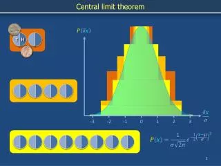
7. Distribution of 200 digits from Social Security Numbers (Last 4 digits from 50 students) Figure 5-19

9. Distribution of 50 Sample Means for 50 Students Figure 5-20

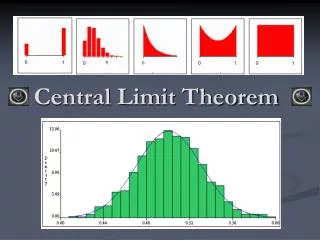
10. As the sample size increases, the sampling distribution of sample means approaches a normal distribution.

11. Example: Given the population of men has normally distributed weights with a mean of 172 lb and a standard deviation of 29 lb, a) if one man is randomly selected, find the probability that his weight is greater than 167 lb.b) if 12 different men are randomly selected, find the probability that their mean weight is greater than 167 lb.

12. z = 167 – 172 = –0.17 29 Example: Given the population of men has normally distributed weights with a mean of 172 lb and a standard deviation of 29 lb, a) if one man is randomly selected, find the probability that his weight is greater than 167 lb.

13. Example: Given the population of men has normally distributed weights with a mean of 172 lb and a standard deviation of 29 lb, a) if one man is randomly selected, the probability that his weight is greater than 167 lb. is 0.5675.

14. Example: Given the population of men has normally distributed weights with a mean of 172 lb and a standard deviation of 29 lb, b) if 12 different men are randomly selected, find the probability that their mean weight is greater than 167 lb.

15. Example: Given the population of men has normally distributed weights with a mean of 172 lb and a standard deviation of 29 lb, b) if 12 different men are randomly selected, find the probability that their mean weight is greater than 167 lb.

16. z = 167 – 172 = –0.60 29 36 Example: Given the population of men has normally distributed weights with a mean of 172 lb and a standard deviation of 29 lb, b) if 12 different men are randomly selected, find the probability that their mean weight is greater than 167 lb.

17. z = 167 – 172 = –0.60 29 36 Example: Given the population of men has normally distributed weights with a mean of 143 lb and a standard deviation of 29 lb, b.) if 12 different men are randomly selected, the probability that their mean weight is greater than 167 lb is 0.7257.

18. b) if 12 different men are randomly selected, their mean     weight is greater than 167 lb.P(x > 167) = 0.7257 Example: Given the population of men has normally distributed weights with a mean of 172 lb and a standard deviation of 29 lb, a) if one man is randomly selected, find the probability     that his weight is greater than 167 lb.P(x > 167) = 0.5675 It is much easier for an individual to deviate from the mean than it is for a group of 12 to deviate from the mean.