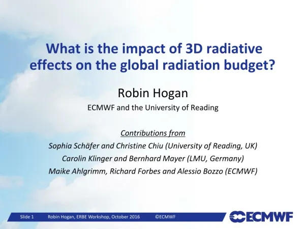
What is the impact of 3D radiative effects on the global radiation budget?
This presentation explores the 3D radiative effects of clouds on the global radiation budget, discussing biases in climate models related to cloud representation. It highlights the complexity of cloud structures, introducing conceptual models and tools like the SPARTACUS solver for improved accuracy. The analysis includes global impacts of 3D radiation on cloud cover and brightness, how cloud heterogeneity affects radiative forces, and offers insights into longwave and shortwave radiative processes, documenting the improvements in model predictions and their implications for climate understanding.

What is the impact of 3D radiative effects on the global radiation budget?
E N D
Presentation Transcript
What is the impact of 3D radiative effects on the global radiation budget? Robin Hogan ECMWF and the University of Reading Contributions from Sophia Schäfer and Christine Chiu (University of Reading, UK) Carolin Klinger and Bernhard Mayer (LMU, Germany) MaikeAhlgrimm, Richard Forbes and AlessioBozzo (ECMWF)
Overview • A puzzling bias • Representing cloud structure in radiation schemes • Conceptual models for 3D cloud-radiation effects • The SPARTACUS solver • How big is a cloud? • An estimate of the global impact of 3D radiation
ECMWF cycle 43R1: clouds in uncoupled model climate Cloud cover: model LWP: model SW CRE: model Cloud cover: MODIS LWP: SSMI SW CRE: CERES-EBAF Cloud cover: difference LWP: difference SW CRE: difference (mean 0.2 W m-2) Cloud cover and LWP are too low, yet clouds are too reflective
“Improvements”: less cloud overlap and less heterogeneity Cloud cover: model LWP: model SW CRE: model Cloud cover: MODIS LWP: SSMI SW CRE: CERES-EBAF Cloud cover: difference LWP: difference SW CRE: difference (mean -3.6 W m-2) Cloud cover is better, SW CRE is worse
2-m temperature bias (winter example) • RMS errors are one way to judge whether a new model version improves forecasts • Mean errors are small but negative and grow during the forecast towards the climatic biases • A related puzzle: global-mean shortwave cloud radiative effect is about right but temperatures are a little low
Most models circa 2000 Model variables needed: cloud fraction, water content Reflection & transmission computed for clear & cloudy regions separately Fluxes merged at layer interfaces according to cloud fraction Plane-parallel, maximum-random overlap
Increases cloud cover and hence magnitude of cloud radiative effect Net impact –1.9 W m-2 at surface and TOA (Shonk & Hogan 2010) Extra input: overlap decorrelation length from cloud radar ~2 km Ground-based (Hogan & Illingworth 2000, Mace & Benson-Troth 2002) CloudSat (Barker 2008, Shonk et al. 2010) Realistic overlap
Cloud structure reduces cloud reflectance Net impact 4.1 W m-2 (TOA), 3.8 W m-2(surf) Cloud water fractional standard deviation ~0.75 Satellite & cloud radar (Barker, Shonk, Cahalan, Oreopoulos, Rossow…) Cloud water overlap decorrelation length ~1 km Ground-based cloud radar (e.g. Hogan & Illingworth 2003) Tripleclouds (Shonk & Hogan 2008)
Info required similar to Tripleclouds but computationally faster Use of stochastic cloud generator leads to some noise in fluxes Now used in many (most?) global weather and climate models Monte-Carlo Independent Column Approximation (McICA) – Pincus et al. (2005)
“It’s better to solve the right problem approximately than the wrong problem exactly,” or “random errors are better than biases.” (for climate!) Use3D cloud distribution generated by a stochastic model in each gridbox How many light rays are needed for random errors to be tolerable? 500? NWP models tolerate random errors much less than climate models Monte Carlo at least provides good benchmark for approximate schemes Full Monte Carlo (being investigated by Barker et al.)
Mechanisms for shortwave 3D effects • Side illumination • Strongest when sun near horizon • Increases chance of sunlight intercepting cloud • Side escape • Strongest for overhead sun • Forward scattering leads to more sunlight penetration • Second-order importance • In-region transport • Systematically reduces reflectance for all solar zenith angles
Idealized calculation: what is the albedo of this scene? R R* R 0 • Surface albedo = 0 • Reflectance of each cloud: R • No absorption so transmittance T = 1 – R R/2 R/2 Independent column approximation • Reflectance of 2 non-absorbing clouds • Adding method with R* = 2R/(1+R) • Reflectance of scene • Weighted average Rscene = R/2 + R*/4 = R(1+R/2)/(1+R) • Optically thick limit: Rscene = 3/4 Horizontal transport in regions • Mean reflectance of layer = R/2 • Reflectance of scene • Random overlap so apply adding method to mean reflectances: Rscene = 2(R/2)/(1+R/2) = 2R/(2+R) • Optically thick limit: Rscene = 2/3
Conceptual model for longwave 3D effects • Radiation can now be emitted from the side of a cloud, increasing downwelling at the surface • A useful benchmark: for an isolated, optically thick, cubic cloud in vacuum, 3D effects increase downwelling flux at the surface by a factor of 3 • Clouds are not cubes, the atmosphere is not a vacuum to longwave radiation: many radiation people assume 3D effects are negligible in the longwave… are they right?
SPARTACUS “Speedy Algorithm for Radiative Transfer through Cloud Sides” va ua a vb ub • Starting point: “Tripleclouds” method • Represent cloud heterogeneity via three regions at each height • Extra terms added to two-stream equations: • Assuming clouds are randomly distributed, we obtain: a b c a b c a New terms representing exchange between regions Length of cloud perimeter per unit gridbox area Fraction of gridbox occupied by clear skies (region a)
Matrix solution in a single layer (shortwave) • Define diffuse upwelling, diffuse downwelling and direct downwelling as vectors u, v and s: • Write two-stream equations as: where 9x9 matrix is composed of known terms analogous to g1-g4 in the standard two-stream equations: • Solution for layer of thickness z1: • Matrix exponential • Waterman (1981), Flatau & Stephens (1998) • Can compute using Padé approximant plus scaling & squaring method (Higham 2005)
Reflection and transmission matrices s(0) v(0) u(0) • We want relationships between fluxes of the form: • Transmission matrix for 2 regions given by: and likewise for R and S± • If matrix exponential is decomposed as: then reflection and transmission matrices given by: • For scalars, get same answer as traditional Meador & Weaver (1980) formulas • For speed, only use matrix exponential for partially cloudy layers u(z1)
Test with I3RC cumulus cloud • Inputs needed by SPARTACUS • Fully 3D simulations with MYSTIC • Thanks to Carolin Klinger & Bernhard Mayer, LMU Munich
Broadband shortwave SPARTACUS vs MYSTIC (Monte Carlo) • Good match! • Big difference in direct surface flux when sun low in the sky Hogan et al. (JGR 2016)
Broadband shortwave SPARTACUS vs MYSTIC (Monte Carlo) • Good match! • Big difference in direct surface flux when sun low in the sky • Change due to in-region horizontal transport • Change due to cloud edge effects Hogan et al. (JGR 2016)
Troccoli & Morcrette (2014) reported biases in ECMWF direct solar radiation from, important for solar energy industry Bin observations and model by solar zenith angle and cloud fraction, considering only cases of boundary-layer clouds (thanks to MaikeAhlgrimm): Next step: apply new 3D radiation scheme to the ECMWF cloud fields to verify that differences are due to 3D effects 3D effects in observations of direct/total downwelling flux ARM SGP (13 yrs) ECMWF model
Longwave… • Good 1D agreement • MYSTIC 3D effect: 30% (the same in broadband) • Too big in SPARTACUS? • Use radiativelyeffective cloud edge length: contour of a fitted ellipse • Consider full cloud field • Effective edge length not sufficient: clustering is also important • We know how to estimate the radiatively relevant edge length; clustering can only be represented approximately (multiply by 0.7 in this case)
How can we characterize cloud edge length in a model? Morcrette (2012): MSG MSG infrared Jensen et al. (2006) data: MODIS stratocumulus Cloud mask
Characterizing cloud perimeter vs. cloud fraction • Jensen et al. (2006) proposed effective cloud diameter D: diameter of identical circular clouds that have the same perimeter and area as the actual cloud field • If cloud area A = p(D/2)2 and perimeter P = pDthen • Effective cloud diameter D = 4A/P = 4x cloud cover / normalized perimeter • Problem with this concept is that effective cloud diameter computed from real cloud fields is strongly dependent on cloud cover • We seek an effective cloud scale S that is independent of cloud cover, and can be parameterized in GCMs Jensen et al. (2006) data: MODIS stratocumulus
Morcrette (2012) • Conceptual model: fill a checkerboard randomly with squares of size S: • Morcrette (2012) found that perimeter simulated in this way behaves the same as in observations: • P = 4A(1-A)/S • His MSG data for all clouds yields S of around 10 km Simulations MSG data
Apply concept to MODIS data • 1-km MODIS is higher resolution than MSG • Application to Jensen et al. stratocumulus data suggests effective cloud scale of around 10 km
Cu & Sc: 1 km (0.7–1.4 range) Approximate account for clustering MODIS too coarse Non-BL clouds: 10 km (5–20 range) Obviously further refinement is needed! Estimates of effective cloud scale (Schäfer 2016, PhD thesis) Sc: I3RC Ci: Hogan & Kew (2005) Cu: Fielding et al. (2014) Cb: Stein et al. (2015)
What is the global impact of 3D radiative transfer? Top of atmosphere Surface • Offline calculations 1 yr of ERA-Interim clouds • Compare McICA to SPARTACUS 3D solver (Hogan et al. 2016) • SW & LW effects both act to warm the surface • Similar order to effect of cloud heterogeneity or doubling CO2 Sophia Schäfer (PhD thesis, 2016) Mean +3.0 W m-2 +2.3 Total Longwave Shortwave +0.9 +2.1 +3.9 +4.4
Comparison of ECMWF model to CERES CRE • Introduction of 3D effects improves agreement with CERES in SW and LW • Is CERES longwave biased compared to model estimates (Allan and Ringer 2003)?
Impact on temperature (8x coupled 1-yr simulations) • Impact on 2-m temperature over land compared to ECMWF IFS control: • Introducing realistic cloud overlap & inhomogeneity: – 0.3 K • Introducing 3D radiation: + 0.4 K (so + 0.7 K due to 3D radiation) – is this the missing physics?
Computational cost inside ECMWF model • New ECRAD radiation scheme with McICA solver is 30-35% faster • ECRAD with SPARTACUS solver: matrix exponential and other matrix operations are the main costsofurther optimization needed
Summary and outlook • New capability to represent 3D radiative effects in a global model • First estimates suggest 4 W m-2 global impact on net fluxes at surface and TOA • Similar to the impact of cloud inhomogeneity and overlap • Longwave effects are significant • Could help explain the cold bias in the ECMWF model? …but many other factors need constraining too! • Further work required: • More analysis of high resolution cloud observations and CRMs to characterize “effective cloud scale” • Comparison of SPARTACUS with full Monte Carlo calculations in a wide variety of scenes • Optimize SPARTACUS: perhaps treat it as a benchmark for more approximate schemes to represent 3D effects, e.g. perturbing cloud overlap (Tompkins & DiGuiseppe) • SPARTACUS is an option in new ECMWF radiation scheme “ECRAD” • Offline version to be released under the OpenIFS license • SPARTACUS idea will also be used to compute 3D effects in urban and vegetation canopies
Do subtle radiative effects really matter for an NWP centre? • Short to medium term • Surface temperature forecasts are of first-order importance • Solar energy industry increasingly using radiation diagnostics from NWP • Monthly to seasonal (both coupled) • Predictability on this timescale from stratosphere, MJO, ocean memory – all require accurate radiation • Difficult to get statistical significance when evaluating different seasonal forecast systems – but a pre-requisite for a skilful system is a model with a good climate Overview • A puzzling bias • Representing cloud structure in radiation schemes • Conceptual models for 3D cloud-radiation effects • The SPARTACUS solver • How big is a cloud? • An estimate of the global impact of 3D radiation
Global impact of cloud inhomogeneity and overlap Top-of-atmosphere cloud radiative forcing Plane-parallel, maximum-random • Fixing just horizontal structure (blue to red) would overcompensate the error • Fixing just overlap (blue to cyan) would increase the error • Need to fix both overlap and horizontal structure Longwave Shortwave Fix only overlap Fix only inhomogeneity Fix overlap and inhomogeneity Shonk & Hogan (2010)
Longwave equivalent • Two-stream equations now look like this: (No solar beam and Planck function assumed to vary linearly in optical depth via inhomogeneous terms) • Solution is a bit more complex: where:
Extension to multiple layers: the adding method • The adding method (e.g. Lacis and Hansen 1974) can be used to combine the reflectance and transmittance matrices of pairs of layers • In N-stream radiative transfer (e.g. N=16), the elements of the flux vector would represent different streams, but the method works just as well for different regions • We work up from the surface and compute the albedo of the whole atmosphere below each half-level • Albedo • After this we can head back down again to compute the fluxes • For one region, this is exactly the same as solving a tridiagonal system with forward elimination followed by backsubstitution Aaa Abb Aab Aba
How do we deal with cloud overlap? • Edwards-Slingo method: overlap matrices • Downward overlap (similarly for upward overlap U) • Matrix elements calculated from a decorrelation length following Shonk et al. (2010) • Albedo just above a half level (A) is related to albedo just below a half level (B) by A=UBV Vaa Vab Vbb Vba Half-level
Schäfer et al. (JGR 2016) What is LW radiatively effective cloud edge length? Single cloud Full cloud field MYSTIC: solid lines SPARTACUS: dashed lines Clustering reduces effective edge length (nearest-neighbour spacing is 280 m vs. random value of 430 m) Ellipses remove radiatively irrelevant small-scale structure “Ellipsified” clouds Original clouds
Clustering has a fairly small effect on atmospheric heating rates 3D effects increaselongwave CRF at surface by 30% in both MYSTIC and SPARTACUS (42% in SPARTACUS if clustering effect not represented) Heating-rate comparisons with MYSTIC Longwave Shortwave
What is the effective size of typical cumulus clouds? • This study: between 0.5 and 1 km • Neggers et al. (2003): cloud resolving model applied to a range of cumulus experiments
Instantaneous cloud radiative forcing applying SPARTACUS to one ERA-Interim clouds To get cloud edge length, assume cumulus horizontal length scale is 750-m, all other clouds 10 km Towards a global estimate of the impact of 3D effects Solar zenith angle Night-time: positive LW effect High sun: positive SW effect Low sun: negative SW effect
Effective size of deep convection (Stein et al., BAMS 2015) • Radar observations suggest cores of UK storms around 10 km wide • Don’t trust size of storms in models with grid spacing larger than around 1 km (Met Office model in this case)