The Wave Model
The Wave Model. ECMWF, Reading, UK. Lecture notes can be reached at:.


The Wave Model
E N D
Presentation Transcript
The Wave Model ECMWF, Reading, UK
Lecture notes can be reached at: http://www.ecmwf.int- News & Events- Training courses - meteorology and computing- Lecture Notes: Meteorological Training Course- (3) Numerical methods and the adiabatic formulation of models- "The wave model". May 1995 by Peter Janssen(in both html and pdf format) Direct link:http://www.ecmwf.int/newsevents/training/rcourse_notes/NUMERICAL_METHODS/ The Wave Model (ECWAM)
Description ofECMWF Wave Model (ECWAM): Available at: http:// www.ecmwf.int- Research- Full scientific and technical documentation of the IFS- VII. ECMWF wave model(in both html and pdf format) Direct link:http://www.ecmwf.int/research/ifsdocs/WAVES/index.html The Wave Model (ECWAM)
Directly Related Books: • “Dynamics and Modelling of Ocean Waves”. by: G.J. Komen, L. Cavaleri, M. Donelan, K. Hasselmann, S. Hasselmann, P.A.E.M. Janssen. Cambridge University Press, 1996. • “The Interaction of Ocean Waves and Wind”. By: Peter Janssen Cambridge University Press, 2004. The Wave Model (ECWAM)
Introduction: • State of the art in wave modelling. • Energy balance equation from ‘first’ principles. • Wave forecasting. • Validation with satellite and buoy data. • Benefits for atmospheric modelling. The Wave Model (ECWAM)
earthquake Forcing: moon/sun wind Restoring: gravity surface tension Coriolis force 2 1 10.0 1.0 0.03 3x10⁻³ 2x10⁻⁵ 1x10⁻⁵ Frequency (Hz) What we are dealing with? The Wave Model (ECWAM)
Water surfaceelevation, Wave Period, T Wave Length, Wave Height, H What we are dealing with? The Wave Model (ECWAM)
What we are dealing with? The Wave Model (ECWAM)
What we are dealing with? The Wave Model (ECWAM)
What we are dealing with? The Wave Model (ECWAM)
What we are dealing with? The Wave Model (ECWAM)
What we are dealing with? The Wave Model (ECWAM)
What we are dealing with? The Wave Model (ECWAM)
What we are dealing with? The Wave Model (ECWAM)
What we are dealing with? The Wave Model (ECWAM)
What we are dealing with? The Wave Model (ECWAM)
What we are dealing with? The Wave Model (ECWAM)
What we are dealing with? The Wave Model (ECWAM)
What we aredealing with? The Wave Model (ECWAM)
What we are dealing with? The Wave Model (ECWAM)
Energy, E,of a single component Simplified sketch! Fetch, X, or Duration, t What we are dealing with? The Wave Model (ECWAM)
Program of the lectures: 1. Derivation of energy balance equation 1.1. Preliminaries- Basic Equations- Dispersion relation in deep & shallow water.- Group velocity.- Energy density.- Hamiltonian & Lagrangian for potential flow.- Average Lagrangian.- Wave groups and their evolution. The Wave Model (ECWAM)
Program of the lectures: 1. Derivation of energy balance equation 1.2. Energy balance Eq. - Adiabatic Part - Need of a statistical description of waves: the wave spectrum.- Energy balance equation is obtained from averaged Lagrangian.- Advection and refraction. The Wave Model (ECWAM)
Program of the lectures: 1. Derivation of energy balance equation 1.3. Energy balance Eq. - Physics Diabetic rate of change of the spectrum determined by: - energy transfer from wind (Sin) - non-linear wave-wave interactions (Snonlin) - dissipation by white capping (Sdis). The Wave Model (ECWAM)
Program of the lectures: 2. The WAM Model WAM model solves energy balance Eq. 2.1. Energy balance for wind sea - Wind sea and swell.- Empirical growth curves.- Energy balance for wind sea.- Evolution of wave spectrum.- Comparison with observations (JONSWAP). The Wave Model (ECWAM)
Program of the lectures: 2. The WAM Model 2.2. Wave forecasting - Quality of wind field (SWADE).- Validation of wind and wave analysis using ERS-1/2, ENVISAT and Jason altimeter data and buoy data.- Quality of wave forecast: forecast skill depends on sea state (wind sea or swell). The Wave Model (ECWAM)
Program of the lectures: 3. Benefits for Atmospheric Modelling 3.1. Use as a diagnostic tool Over-activity of atmospheric forecast is studied by comparing monthly mean wave forecast with verifying analysis. 3.2. Coupled wind-wave modelling Energy transfer from atmosphere to ocean is sea state dependent. Coupled wind-wave modelling. Impact on depression and on atmospheric climate. The Wave Model (ECWAM)
Program of the lecture: 4. Tsunamis 4.1. Introduction- Tsunami main characteristics.- Differences with respect to wind waves. 4.2. Generation and Propagation- Basic principles.- Propagation characteristics.- Numerical simulation. 4.3. Examples- Boxing-Day (26 Dec. 2004) Tsunami.- 1 April 1946 Tsunami that hit Hawaii The Wave Model (ECWAM)
1. Derivation of the Energy Balance Eqn: Solve problem with perturbation methods:(i) a / w << 1 (ii) s << 1 Lowest order: free gravity waves. Higher order effects: wind input, nonlinear transfer & dissipation The Wave Model (ECWAM)
Deterministic Evolution Equations • Result: Application to wave forecasting is a problem: 1. Do not know the phase of waves Spectrum F(k) ~ a*(k) a(k) Statistical description 2. Direct Fourier Analysis gives too many scales: Wavelength: 1 - 250 m Ocean basin: 107 m 2D 1014 equations Multiple scale approach · short-scale, O(), solved analytically · long-scale related to physics. Result: Energy balance equation that describes large-scale evolution of the wave spectrum. The Wave Model (ECWAM)
1.1. Preliminaries: • Interface between air and ocean: • Incompressible two-layer fluid • Navier-Stokes:Here and surface elevation follows from: • Oscillations should vanish for:z± and z = -D (bottom) • No stresses; a 0 ; irrotational potential flow: (velocity potential )Then, obeys potential equation. The Wave Model (ECWAM)
Laplace’s Equation • Conditions at surface: • Conditions at the bottom: • Conservation of total energy: with The Wave Model (ECWAM)
Hamilton EquationsChoose as variables: and Boundary conditions then follow from Hamilton’s equations:Homework: Show this!Advantage of this approach: Solve Laplace equation with boundary conditions: = (,). Then evolution in time follows from Hamilton equations. The Wave Model (ECWAM)
Lagrange FormulationVariational principle:with:gives Laplace’s equation & boundary conditions. The Wave Model (ECWAM)
V(q) • IntermezzoClassical mechanics: Particle (p,q) in potential well V(q)Total energy: Regard p and q as canonical variables. Hamilton’s equations are: Eliminate p Newton’s law = Force The Wave Model (ECWAM)
Principle of “least” action. Lagrangian:Newton’s law Action is extreme, whereAction is extreme if (action) = 0, where This is applicable for arbitrary q hence (Euler-Lagrange equation) The Wave Model (ECWAM)
Define momentum, p, as:and regard now p and q are independent, the Hamiltonian, H , is given as:Differentiate H with respect to q givesThe other Hamilton equation:All this is less straightforward to do for a continuum. Nevertheless, Miles obtained the Hamilton equations from the variational principle.Homework: Derive the governing equations for surface gravity waves from the variational principle. The Wave Model (ECWAM)
Linear TheoryLinearized equations become:Elementary sineswhere a is the wave amplitude, is the wave phase.Laplace: The Wave Model (ECWAM)
Constant depth: z = -DZ'(-D) = 0Z ~ cosh [ k (z+D)] with Satisfying Dispersion RelationDeep waterShallow waterDD0 dispersion relation: phase speed: group speed: Note: low freq. waves faster! No dispersion. energy: The Wave Model (ECWAM)
(t) t Slight generalisation: Slowly varying depth and current, , = intrinsic frequency • Wave GroupsSo far a single wave. However, waves come in groups.Long-wave groups may be described with geometrical optics approach:Amplitude and phase vary slowly: The Wave Model (ECWAM)
Local wave number and phase (recall wave phase !) Consistency: conservation of number of wave crests Slow time evolution of amplitude is obtained by averaging the Lagrangian over rapid phase, .Average L: For water waves we getwith The Wave Model (ECWAM)
In other words, we have Evolution equations then follow from the average variational principle We obtain:a : : plus consistency: Finally, introduce a transport velocity thenL is called the action density. The Wave Model (ECWAM)
Apply our findings to gravity waves. Linear theory, write L aswhere Dispersion relation follows fromhence, with , Equation for action density, N ,becomeswith Closed by The Wave Model (ECWAM)
Consequencies Zero flux through boundaries hence, in case of slowly varying bottom and currents, the wave energy is not constant. Of course, the total energy of the system, including currents, ... etc., is constant. However, when waves are considered in isolation (regarded as “the” system), energy is not conserved because of interaction with current (and bottom). The action density is called an adiabatic invariant. The Wave Model (ECWAM)
Homework: Adiabatic Invariants(study this) Consider once more the particle in potential well. Externally imposed change (t). We have Variational equation is Calculate average Lagrangian with fixed. If period is = 2/ , then For periodic motion ( = const.) we have conservation of energythus also momentum is The average Lagrangian becomes The Wave Model (ECWAM)
Allow now slow variations of which give consequent changes in E and . Average variational principle Define again Variation with respect to E & gives The first corresponds to the dispersion relation while the second corresponds to the action density equation. Thus which is just the classical result of an adiabatic invariant. As the system is modulated, and E vary individually but remains constant: Analogy LL waves. Example: Pendulum with varying length! The Wave Model (ECWAM)