Download
1 / 1
10 likes | 105 Vues
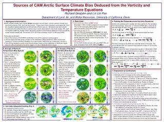
Study on Arctic surface bias in CAM climate model, analyzing local and remote mechanisms using 3-D modeling and observational data.

E N D
Sources of CAM Arctic Surface Climate Bias Deduced from the Vorticity and Temperature Equations Richard Grotjahn and Lin Lin Pan Department of Land, Air, and Water Resources, University of California, Davis 2. Data Used 3. Parsing the Temperature and Vorticity Equations 1. Background Information Linear Stationary Wave (LSW) Model Branstator (1990) model is adapted to this problem. The model linearizes CAM primitive equations about the winter (DJF) time mean. Observational data (DJF) We use ERA-40 reanalysis (“ERA data”) 4x daily data from 12/1979 to 2/2002. Data are imported at full resolution then regridded to match the LSW model resolution when constructing the bias. Ps is from NCEP reanalysis. CAM3 data (DJF) On the UCD cluster we ran a 20 year AMIP T42, 23 level, simulation from 1979-1998 of CAM3.0. • NCAR climate models have similar winter simulation errors (bias) in Arctic surface climate (e.g. sea level pressure, SLP, and low-level wind). These errors have important consequences, such as unrealistic spatial distribution and thickness of Arctic sea ice. We study local and remote mechanisms that affect the Arctic surface bias in both observations and model output. We used uncoupled (CAM 3.0) model output, since the coupled runs introduce additional error brought by ocean model climate drift. The winter (DJF) SLP bias is similar in both CCSM and CAM3. • Previously we showed: • The 3-D structure of the CAM3 model bias in the Arctic and surrounding region. • The forcing of the bias using a model of the linearized CAM3 dynamics. (With friction and heating to control nonlinear instability the model treats CAM3 bias as a stationary ‘solution’.) • The forcing needed to produce the structures and nearly all the amplitude of the Arctic region bias are either localized to the Arctic region or in the midlatitude storm tracks. Define time average with overbar and use a prime for the deviation from that average. Subscript “C” denotes CAM3 data; subscript “E” denotes ERA-40 data. The time mean of the CAM3 model data is: For the time mean of the ERA-40 observational data we have: Define a ^ notation for the bias. Subtract: (1) – (2) to obtain: The first 2 terms on the RHS are nonlinear terms in the bias. The group labeled THF are transient heat advection bias. Q^ is the bias in diabatic heating. One can solve time mean temperature equation in Branstator LSW model to find T^ from specified forcing or specify T^ to find forcing: 4. Groups of Terms in Temperature Bias Eqn (3) 5. Groups of Terms in Vorticity Bias Eqn (5) • Terms in (3) at levels σ= 0.5, and 0.95; σ=1 is Earth’s surface. Calculated in T42 plotted at R12. • Term 1: linear advection terms by the stationary bias and climatological fields; it is all terms on the LHS of (3). • Term 2: nonlinear advection of the bias by the bias; it is the first 2 terms on the RHS of (3). • Term 3: time mean advection by the transients; it is labeled THF in (3). • Term 4: diabatic heating bias, Q^. Only high frequency (2-8 days) transient parts of Q^. • Terms in (5) at levels; σ= 0.5, and 0.95; where σ=1 is Earth’s surface. Calculated in T42 plotted at R12. • Term 1: linear advection terms by the stationary bias and climatological fields; it is all terms on the LHS of (5). • Term 2: nonlinear advection of the bias by the bias; it is the first 4 terms on the RHS of (5). • Term 3: time mean advection by the transients; it is all primed terms in (5). • Term 4: F^ bias of diffusion/friction. F is for nonlinear bias, quadratic transient advection and diabatic processes. When run in reverse, the LSW model finds F (for all 4 governing equations: T, D, ζ, and q=lnPs.) Similar to (3), the vorticity bias equation is 7. Discussion & Conclusions • Forcing of Temperature bias, eqn (3), Figs. 1 & 2. • LSW bias (term 1) is larger of the terms at upper levels. • Dipolar in Atlantic & Europe (negative NW of positive); • >0 over W. Siberia; <0 below, >0 above for E. Siberia & Alaska. • Nonlinear (term 2) is comparable to term1 only near ground: • At σ=0.95 mostly <0 over Scandinavia, Russia, & Alaska. • Transients (term 3) comparable to term 1 at upper levels a few locs. • At σ=0.5: >0 over Scandinavia, <0 N. Pacific • At σ=0.95: dipolar along Pacific coast; opposes term 1 over land. • Diabatic (term 4) large at upper and surface levels; • large and <0 over most of Arctic (>65N) • >0 along Atlantic storm track, <0 at start of Pacific storm track • Transient & diabatic forcing key at surface & Atlantic storm track. • B. Forcing of Vorticity bias, eqn (5), Figs. 3 & 4. • Linear (term 1) very noisy, dominates at upper levels and surface. • Transients (term 2) <0 along storm tracks (CAM vorticity flux too big) • Friction term dominates at surface • C. Vertically-integrated heating bias results, Fig. 5. • Q1 dominated by heating bias (>0) over Atlantic, Pacific, W. coast • Net radiative cooling bias over Arctic Ocean, • >0 over Atlantic storm track & Russia mainly Precip., also Rad. • Pacific storm track <0 at start from SHF, >0 at end from P & R. • D. Conclusions from Temperature (3) and Vorticity bias (5) results • Analyses of (3) and (5) justify use of linear LSW to study bias. • Storm tracks different impacts, N. Atlantic more import to Arctic bias. • Near-surface biases of most terms over Arcitc may be important. Fig. 3: Term 1 (top), term 2 (middle), term 3 (bottom) Contour values and intervals vary. Fig. 1: Term 1 (top), term 2 (middle), term 3 (bottom) Fig. 2: Term 4 transient diabatic heating bias Fig. 4: Term 4 Friction bias 6. Vertically-integrated heating (Fig. 5) • See Trenberth & Smith (2008) • A) Vertically-integral latent heating (L*P) bias • B) Surface sensible heat flux (SHF) bias • C) Top of atmosphere net radiation (R) bias • D) Total heating: Q1 = R+SHF+LP • E) Moisture eqn implied heating: Q2=L*(P-E) • F) Total energy eqn heating: Q1 – Q2