Download
1 / 31
310 likes | 355 Vues
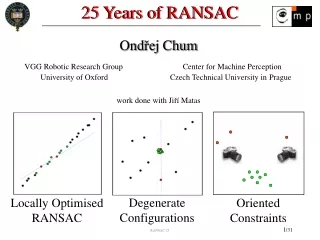
Explore the evolution of RANSAC, focusing on locally optimized solutions and hierarchical model estimation. Discover improved methods for handling degenerate configurations and achieving robust fittings in both toy and real-world examples.

E N D
25 Years of RANSAC 25 Years of RANSAC Ondřej Chum VGG Robotic Research Group Center for Machine Perception University of Oxford Czech Technical University inPrague work done with Jiří Matas DegenerateConfigurations OrientedConstraints Locally OptimisedRANSAC RANSAC 25
Locally optimised RANSAC Chum, Matas, Kittler: Locally Optimized RANSAC, DAGM , 2003 Chum, Matas, Obdržálek: Enhancing RANSAC by Generalized Model Optimization, ACCV, 2004 RANSAC 25
The Stopping Criterion ... • Observation: often, the solution is found later than predicted, i.e. after on average k steps where is the fraction of inliers, m the sample size • RANSAC stopping criterion makes a (hidden) assumption that an all-inlier sample leads to the solution. RANSAC 25
.... Makes an Invalid Assumption Not every all-inlier sample gives a model consistent with all inliers Lower number of inliers is detected RANSAC runs longer RANSAC 25
Solution: Local Optimisation Step Repeat k times 1. Hypothesis generation 2. Model verification 2b. If model best-so-far Execute (Local) Optimisation Inner RANSAC + Re-weighted least squares:- Samples are drawn from the set of data points consistent with the best-so-far hypothesis - New models are verified on all data points - Samples can contain more than minimal number of data points since consistent points include almost entirely inliers How often? Conclusion: the LO step 2b is executed rarely, does not influence runing time significantly RANSAC 25
Validation: Two-view Geometry Estimation Histograms of the number of inliers returned over 100 executions of RANSAC (top) and LO-RANSAC (bottom) Result: (i) variation of the number of inliers significantly reduced (ii) speed-up up to 3 times (for 7pt EG and 4pt homography est.) RANSAC 25
LO: Hierarchical Model Estimation A model from a random sample need not be required to be the solution. Any model that is consistent with a large proportion of inliers moves us closer to a solution, since its inliers can be sampled. Idea: • Estimate approximate models with lower complexity (less data points in the sample) with loose thresholds • Followed by LO step estimating full model RANSAC 25
Estimation via Approximate Models • Epipolar geometry and radial distortion • Standard: • 9 point correspondences define the model • LO Ransac: • Approximated by EG with no radial distortion • In LO step (2b), estimate the full model from 9 (or more!) points Division modelFitzgibbon CVPR’01 EG from 3 local affine frame (LAF) correspondences- each region provides 3 points - 3 LAFs determine EG - points close to each other (low precision) Chum, Matas, Obdržálek: Enhancing RANSAC by Generalized Model Optimization, ACCV 2004 RANSAC 25
Radial Distortion I RANSAC 25
Radial Distortion II RANSAC 25
EG from Three Correspondences More than 10000-fold speed-up RANSAC 25
SUMMARY • Not every all-inlier sample generates model consistent with all inliers due to noise • Local data driven search initialised by the best-so-far solution saves computational effort • Using hierarchical estimation (starting with approximate models) speeds up the estimation EG from Three Correspondences More than 10000-fold speed-up RANSAC 25
Degenerate Configurations Chum, Werner, Matas: EG Estimation unaffected by dominant plane, CVPR’05 RANSAC 25
Degenerate Configurations • Infinite number of models passes through a degenerate configuration • Sample with points from both the degenerate configuration and outlier(s) is a problem – it has higher than random support RANSAC 25
Toy Example • Robust fitting of a plane to 3D points • Algorithm: • Draw samples of three points & fit a plane to them • Calculate the support of the plane Problem: • High number of points lie on a line • A sample containing two points from the line and one outlier has large support (the whole line) • Such sample is not degenerate, the problem does not show as a singularity in the model estimation step • Algorithm may return incorrect plane (that contains the line) RANSAC 25
Real Example The Dominant Plane Problem: Given many (almost) coplanar points, a few points off the plane, and (possibly) many outliers estimate the epipolar geometry (EG), if possible. RANSAC run with 95% confidence actually finds the inliers on the lamppost in only 17% of executions RANSAC 25
In the Presence of a Dominant Plane • RANSAC draws minimal samples of 7 correspondences to hypothesize the epipolar geometry • When dominant plane is present, samples with more than 4 coplanar correspondences often appear • 7 or 6 coplanar correspondences: the sample is consistent with a family of fundamental matrices. This case is easily be detected. • Chum et al. CVPR’05 show that the epipolar geometry hypothesised from 5 coplanar points from the dominant plane and 2 off the plane (a so called H-degenerate sample) has a large RANSAC support. If at least one of the off-plane correspondences is an outlier, the EG is incorrect. RANSAC 25
Different Solutions Returned by RANSAC RANSAC 25
DEGENSAC Core of the algorithm: • Draw samples of 7 correspondences and estimate 1-3 fundamental matrices by the 7-point algorithm • Test samples with the largest support so far for H-degeneracy • When H-degeneracy was detected, use plane-and-parallax algorithm [Irani&Anadan ECCV’97]. Note: the plane-and-parallax needs to draw samples of only 2 correspondences to hypothesize EG, therefore its complexity is negligible compared to RANSAC where 7 correspondences are drawn into a sample Alternative to step 2: execute RANSAC detecting degenerate configuration on inliers: Frahm, Pollefeys: RANSAC for (Quasi-)Degenereate Data (QDEGSAC), CVPR’06 RANSAC 25
Stability of the Results How many times will a correspondence be labeled as an inlier, if we run the experiment 100 times? Off the plane correspondences RANSAC DEGENSAC Correspondence number RANSAC 25
Exploiting Non-minimal Samples I Finding collinear sets of 3D points via plane fitting Assumption: Outliers are uniformly distributed in 3D Algorithm: • Draw samples of three points & fit a plane to them • Calculate the support of the plane • Check the three lines defined by the points of samples with the largest support so far Advantage: it is more likely to draw at least 2 inliers out of 3 than 2 out of 2 when fitting a line Disadvantage: does not work if all points occupy a single plane RANSAC 25
Exploiting Non-minimal Samples II Finding homographies via EG fitting Ratio of the number of samples needed to estimate homography by drawing samples of four and seven correspondences respectively Probability of drawing 4 inlierers P2 / P1 Probability of drawing a 7-tuple with at least 5 inliers Fraction of inliers RANSAC 25
SUMMARY • Mixed samples of data from degenerate configuration and outliers result in incorrect estimates • Detecting the degeneracy and using it to guide the search avoids the problem and can speed the estimation process up • Drawing non-minimal samples can be more efficient than drawing minimal samples! Exploiting Non-minimal Samples II Finding homographies via EG fitting Ratio of the number of samples needed to estimate homography by drawing samples of four and seven correspondences respectively Probability of drawing 4 inlierers P2 / P1 Probability of drawing a 7-tuple with at least 5 inliers Fraction of inliers RANSAC 25
Oriented Constraintsin RANSAC Chum, Werner, Matas: Epipolar geometry estimation via RANSAC benefits from the oriented epipolar constraint, ICPR’04 RANSAC 25
Additional Constraints • Constraints on the model parameters that do not reduce the model complexity (the number of data points that define the model ‘uniquely’) exist in some problems. • Possible approaches: • Sample so that only hypotheses satisfying the constraints are generated • may be time demanding or even intractable • Ignore additional constraints • typically works OK since models that are not allowed do not have sufficient support • Check the constraints before verification step • can save a lot of time on verification RANSAC 25
Constraints on Two-View Geometry Cameras can only observe points in front of the camera – rays are half-lines Oriented projective geometry Stolfi [’91] Laveau and Faugeras [ECCV ’96] Werner and Pajdla [ICCV’98, BMVC’01] RANSAC 25
Orientation Constraints for Homography • The test reduces to comparing signs of two determinants (four times) • Can be performed prior to computing the homography RANSAC 25
Oriented Epipolar Geometry • Algorithm: • Draw sample of seven points • Estimate fundamental matrices • Check, whether the oriented constraint holds for all 7 correspondences in the sample • The test takes only 27 – 81 floating point operations Oriented epipolar geometryis a stronger constraint thanunoriented one RANSAC 25
Experimental Results 500,000 samples drawn RANSAC 25
SUMMARY It pays off to apply all available constraints. Experimental Results 500,000 samples drawn RANSAC 25
END RANSAC 25