Option Pricing Models
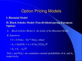
Option Pricing Models. I. Binomial Model II. Black-Scholes Model (Non-dividend paying European Option) A. Black-Scholes Model is the Limit of the Binomial Model B. Equations C = S N(d 1 ) - Xe -rT N(d 2 ), where d 1 = [ln(S/X) + (r + 0.5 S 2 )T]/ S T d 2 = d 1 - S T

Option Pricing Models
E N D
Presentation Transcript
Option Pricing Models • I. Binomial Model • II. Black-Scholes Model (Non-dividend paying European Option) • A. Black-Scholes Model is the Limit of the Binomial Model • B. Equations • C = S N(d1) - Xe-rT N(d2), where • d1 = [ln(S/X) + (r + 0.5S2)T]/ST • d2 = d1 - ST • N(d1), and N(d2) are cumulative normal probabilities of d1 and d2, respectively.
Factors that determine the option value • Underlying stock price • Exercise price • Time to expiration • Interest rate • Underlying stock volatility
Example : B-S Option Pricing S = $98 ; X = $100 r = 0.05 (continuously compounded annual risk-free rate) T = 0.25 (one quarter of a year) S = 0.5 (Annual standard deviation of the continuously compounded stock returns) d1 = [ln(S/X) + (r + 0.5S2)T]/ST = [ln(98/100) + (0.05 + 0.5(0.25))(0.25)] / 0.5(0.5) = 0.0942 d2 = d1 - ST = 0.0942 - (0.5) 0.25 = -0.1558 N(d1) = N(0.0942) N(0.09) = 0.5359
N(d2) = N(-0.1558) N(0.15) = 0.5596 N(-0.15) = 1 - 0.5596 = 0.4404 Excel: normsdist( ) N(d1) = N(0.0942) = 0.5375 N(d2) = N(-0.1558) = 0.4381 C = S N(d1) - Xe-rT N(d2) = (98) (0.5375) - 100 e -0.05 (0.25) (0.4381) = $9.41 OPTION CALCULATOR
B. Hedge Ratio • = C / S = N(d1) • III. More about the model inputs • A. Underlying stock price • B. Time to Expiration • C. The Risk-free Rate: continuously compounded risk-free rate • D. Volatility • Expected Volatility • Proxy: Historical Volatility
Variance of continuously compounded returns • 1. Calculate continuously compounded returns: rS = ln(1+RS), • or, rs = ln(Pt/Pt-1) • 2. Calculate standard deviation S • 3. Annualized standard deviation • Example • CBOE Historical Volatility
F. Historical Volatility and Implied Volatility • represents expected volatility of the stock over the life of the option. • Historical provides estimates of the future volatility. • Implied volatility is the market’s estimates of the stock volatility. • Option traders can compare their own expectations of future price volatility with the implied price volatility. If these are not consistent with one another, the option price may be wrong.
Estimation of implied volatility • IV. Relationship between Model Inputs and Call Price • A. Delta • d = C / S = N(d1) • = f (S) • = f (T) • Delta is the hedge ratio • Position Delta – the sum of the deltas • long 10,000 shares of stock, short 63 calls with = 0.377, long 134 puts with = -0.196 • Position Delta = 10,000 (1) + (-63) (100) (0.377) + 134 (100) (-0.196) • = 4,998.5 • Meaning: total portfolio is equivalent in market risk of 4,998 shares of stocks
B. Gamma • = / S • For stock-option hedgers, the value of measures the extent to which a change in the stock price will force a revision in the hedge ratio. • = f(S) • = f(T) • C. Rho • • = C / i • This is a liner relationship; the impact of changes in i on changes in C normally is small.
D. Vega = C / s = f (S) E. Theta = C / T Theta is a measurement of the rate of time value decay. = f(S)
V. Put Option Pricing • A. Equations • P = -S [1-N(-d1)] + Xe-rT [1-N(-d2)], where • d1 = [ln(S/X) + (r + 0.5S2)T]/ST • d2 = d1 - ST
Homework • 1. Calculate B-S call price for INTC using Friday’s closing stock price and a X that is most close to S. (Use Excel, not manual calculation) • Calculate three implied volatility – one near at-the-money call, one deep out-of-the-money call, and one deep in-the-money call. Draw a diagram relating these three implied volatility and option moneyness. • Calculate 6 “Vegas” assuming six different stock prices. Plot these six “Vegas” against six stock prices.