Option pricing models
Learn to estimate the market value of option contracts using two fundamental models: the Binomial Model and the Black-Scholes Model. This guide delves into the one- and two-period binomial models, with practical examples illustrating how to calculate the price of call options and create risk-free portfolios. Additionally, discover the Black-Scholes formula, including a step-by-step calculation of theoretical call option values. Enhance your financial acumen with easy-to-understand explanations, making these concepts accessible for both novice and experienced investors.


Option pricing models
E N D
Presentation Transcript
Objective Learn to estimate the market value of option contracts.
Outline • The Binomial Model • The Black-Scholes pricing model
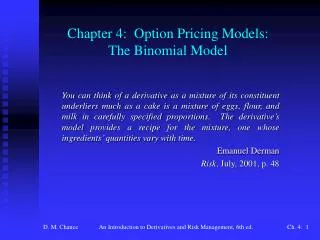
The Binomial Model A very simple to use and understand lattice model that provides the theoretical foundation for other, more advanced models
The one-period binomial model Exemplification Assume the stock of ABC currently sells for $100/share. A call option on the ABC is struck at $120/share and expires in one year. In one year, the stock can either go up by 50% or down by 25%. How much should you pay for the call today if the risk free rate is 10%?
The one-period binomial model: A hedged portfolio Question: Can we combine the call option and the stock in a risk-free portfolio? Yes. Buy 4 shares of stock and sell 10 call options.
A hedged portfolio Su = $150 1+ u = 1.5 Portfolio value: $150(4) - $30(10) = $300 S0 = $100 Buy 4 shares and sell 10 calls Cash flow = 10C0 - $400 1+ d = 0.75 Sd = $75 Portfolio value: $75(4) = $300
A hedged portfolio: Summary Our portfolio is risk-free. We invested 10C0 - $400 and we obtained $300 over one year Our portfolio must earn the risk-free rate. (10C0 - $400)(1.1) = $300 C0 = $12.73 The call option on stock ABC, struck at $120 and expiring in one year, should sell today for $12.73
How did we know to buy 4 shares and write 10 calls?Calculating the hedge ratio, h We required that the value of the portfolio stays the same regardless of the stock price: -Cu + h(1+u)S0 = -Cd + h(1+d)S0 h = the ratio of number of shares to number of calls h =(Cu - Cd)/(Su - Sd) In our case: h =($30 - $0)/$100(1.5 - 0.75) =0.4
The one-period binomial model It follows that: (hS0 - C0)(1+r) = h(1+d)S0 - Cd C0 = [h(1+r)S0 + Cd - h(1+d)S0]/(1+r) Remember, h =(Cu - Cd)/(Su- Sd) C0 = [(Cu - Cd)/(Su-Sd) (1+r)S0 + Cd - (Cu - Cd)/(Su-Sd) (1+d)S0]/(1+r)
The one-period binomial model C0 = [pCu + (1-p)Cd]/(1+r) where p = (r-d)/(u-d) 1 - p = (u-r)/(u-d)
The two-period binomial model Exemplification Assume the stock of ABC currently sells for $100/share. A call option on the ABC is struck at $120/share and expires in twoyears. Each year, the stock can either go up by 50% or down by 25%. How much should you pay for the call today if the risk free rate is 10%?
The two-period binomial model Suu = $225 1+ u = 1.5 Su = $150 1+ u = 1.5 1+ d = 0.75 Sud = $112.50 S0 = $100 1+ u = 1.5 1+ d = 0.75 Sd = $75 1+ d = 0.75 Sdd = $56.25
The two-period binomial model C0 = [p2Cuu +2p(1-p)Cud + (1-p)2Cdd]/(1+r)2
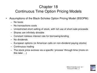
What if we have n-periods? Assume Returns are log-normal distributed The risk-free rate and the returns volatility are constant Each period becomes extremely short Interest is compounded continuously No transaction costs The options are European and/or American but no dividend is paid on the stock until after expiration
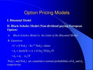
The Black-Scholes formula C = SN(d1) - Ee-rT N(d2) S = current stock price E = exercise price d1 = [ln(S/E) + (r + 2/2)T]/ T1/2 d2 = d1 - T1/2 N(d1), N(d2) = cumulative normal probabilities = annualized standard deviation of stock’s return r = continuously compounded risk-free rate T = time to maturity
The Black-Scholes formula: A numerical example Digital Equipment July 165 call has 35 days to maturity (assume 365 days in a year) The current stock price is $164 The risk-free rate is 5.35% The standard deviation of the return is 29% Calculate the theoretical value of the call option
Step 1 Express the risk-free rate as a continuously compounded yield (find out that continuously compounded rate that would yield 5.35%): (1 + r*/n)n = 1.0535 er* = 1.0535 r* = ln(1.0535) = 0.0521
Step 2 Calculate d1 and d2: d1 = [ln(164/165) + (0.0521 + 0.0841/2)0.0959]/(0.29)(0.309677) d1 = [ - 0.006079 + 0.009029 ]/(0.0898063) = 0.0328485 d2 = 0.0328485 - 0.0898063 = - 0.0569578
Normal distribution table: p(x < z-statistic)
Step 3 N(0.03) = 0.5 + 0.012 = 0.512 N(-0.06) = 0.5 - 0.0239 = 0.4761
Step 4 C = 164(0.512) - 165e-(0.521)(0.0959)(0.4761) C = 83.968 - 165(0.995)(0.4761) = $5.803
Discussion Right now, the stock is at $164 The call is out-of-the-money (intrinsic value is zero) The market value should be $5.803, reflecting the probability that, by expiration, the stock price might increase This probability calculation is based on observing the volatility of return
Relationship between several variables and the market value of options
Relationship between several variables and the market value of options
Relationship between several variables and the market value of options
Relationship between several variables and the market value of options
Relationship between several variables and the market value of options
Relationship between several variables and the market value of options