Download

1 / 47
490 likes | 1.04k Vues
A Heightfield on an Isometric Grid. A Heightfield on an Isometric Grid. Morgan McGuire and Peter Sibley Brown University. The Isometric Heightfield. 10% more accurate, subjectively smoother Practical for real applications GPU accelerated Drawback: requires resampling. Motivation.

E N D
A Heightfield on an Isometric Grid A Heightfield on an Isometric Grid Morgan McGuire and Peter Sibley Brown University
The Isometric Heightfield • 10% more accurate, subjectively smoother • Practical for real applications • GPU accelerated • Drawback: requires resampling
Traditional Ortho-Heightfield Grid 3D View y-displacement
Heightfield Benefits • Represent scientific data at highest fidelity • Practical • Great for dynamic data • Storage efficient for high-frequency data • Simple!
Worst Case Ortho Fit vs. Best
Musgrave’s Heightfield • Shear axes to produce a parallelogram • Equilateral tessellation Grid Space World Space c x r z
x z New Isometric Heightfield • New Mapping • Shift odd rows ½ edge length • Slide end vertices to make square tiles • Border padding for computing vertex normals • Drop-in replacement for ortho-heightfield Grid Space World Space r c
Related Work • Musgrave 88 • Grid Tracing: Fast Ray Tracing for Height Fields • Duchaineau et al 97 • ROAMing terrain: real-time optimally adapting meshes • de Boer 00 • Fast Terrain Rendering Using Geometrical MipMapping • Shankel 02 • Fast Heightfield Normal Calculation • Middleton 01, 02 • Edge Detection in a Hexagonal-image Processing Framework • Markov Random Fields for Square Hexagonal Textures
Signal Processing Analysis • Underlying “true” function h(x, z) • Heightfield approximation: • Low-pass filter and sample • y(x, z) at integer x, z • Barycentric interpolation for non-integer x, z • Reasons for poor fit: • Aliasing from inadequate sampling • Inappropriate reconstruction filter (i.e. triangles)
Experiment • Approximate a 2D Sinusoid h(x, z) = sin(f[x cosq + z sinq ] +f) • Vary phase, angle, and frequency • Error Metrics • Elevation • Shading • Normal deflection • Curvature • Any function is a weighted sum of sinusoids • Draw generalizations about arbitrary functions
Cleaner High Freq. Iso Ortho
Smoother Low Freq. Iso Ortho Shaded
Smoother Low Freq. Iso Ortho Shaded Curvature
Shading Error (lower is better) Isometric: 25% more accurate shading.
Resampling • Existing ortho-grid sampled data • Reconstruct true continuous surface • Filter and downsample on hex pattern • Lossless if original was correctly sampled • Artist created data • Iso-heightfield as modeling primitive
Moving on the Surface • We know elevation at vertices • We need elevation between vertices • Must exactly match rendered elevation! • 4 cases, easily derived from Barycentric interpolation H L=(1-b)H+bI J=(1-b)H + bG P=(1-g)J+gL I G
D E P F I G H Fast Vertex Normals • Indices of neighbors: • Grid space edge vectors: • Vertex normal contains 6 cross-products:
D E P F I G H Fast Vertex Normals • Algebra dramatically simplifies: • Operation count: 6 add, 1 mul • Cheaper than 1 cross-product!
Normals in Vertex Shader • 6 texture lookups (NV50?) • Neighbor indices are the same for each tile • Precompute and store in tex coord stream const uniform mat4 K = vec3 A(tex2D(d), tex2D(h), tex2D(i)); vec3 B(tex2D(g), tex2D(e), tex2D(f)); vec4 C(A – B, 1); vec4 N = mul(K, C); Precomputed outside vertex shader Actual per-vertex work
Heightfield Tiles • Page from disk • Unit of LOD, texturing Wake Island from Battlefield 1942 courtesy of Digital Illusions CE
Triangle Strips Start End
Sub-sampled LOD • Geo-mipmapping would be ideal • Cannot afford to touch vertices on CPU • Use subsampling • Keep edges at maximum resolution • Carefully alpha-blend transitions
Efficient Storage (NV20+) • Pack x, z in int16 vertex stream • Same for every tile • Pack y in int16 texture coordinate stream • Combine streams in vertex shader • Modify y on CPU, upload a relatively small vertex array • 2 bytes/vertex vs. 12 bytes/vertex
Efficient Storage (NV40) • Put y in a texture • SM 3 allows texture lookup in vertex shader! • Modify y using render-to-texture • Navier-Stokes • Render deformations • Tire tracks & footprints • [insert your favorite GPU hack here]
Acknowledgements • Advisor John F. Hughes • Battlefield 1942 data courtesy of Digital Illusions CE • Mars data from Dr. James Head III, Brown University • Additional coding: • Hari Khalsa • Nick Musurca Hardware and data made available by:
Elevation Error (lower is better) Isometric: Same quality with 10% fewer polygons.
What about ROAM? • Irregular tessellation: • y(x, z) for a data-dependent set of samples • Barycentric interpolation between samples • Can produce a better fit • Less aliasing: put samples where needed • e.g. ROAM, Triangulated Irregular Networks • Heightfields are still preferred for many applications…
Our Mapping (2) • Grid to world space: • Grid space to memory: • Row and column sizes: • Also tweak end-vertices on even rows • Drop-in replacement for orthogonal heightfield • Square tiles • Convenient texture & normal mapping
H P I G Need Indices and Weights Indices: g = ?, h = ?, i = ? Weights: wG = ?, wH = ?, wI = ?
H L=(1-b)H+bI J=(1-b)H + bG P=(1-g)J+gL I G Barycentric Interpolation • Simple equations exist for g, h, i, a, b • 4 triangle orientations: {even row, odd row} x {up, down} wG = b(1 – g) = b - a, wH = 1 -b, wI = bg = a
Example • Given P = (c, r) • Let • Example: odd row, up triangle • 3 other cases g = p + C, h = p, i = g +1 b = v, a = u
Self-Shadowing is Hard Problems: • Shadow maps are expensive for terrain • High fill rate • Shadow volumes expensive for terrain • High fill and vertex rate • Pre-computation, horizon map no good for dynamic data
A Trick for Shadowing • Constrain the sun orbit the z-axis • i.e. moves strictly East-West • (x0, z0) only be shadowed by (x0 – k, z0) • Start at the sun end of the x-axis, iterate over vertices • Incrementally compute the max shadowed elevation • Works on ortho-heightfield too
Fast Shadow Volumes • Terrain shadows other objects • Other objects do not shadow terrain (use projective shadows, shadow maps, volumes, etc. for that) • Iterates along rows, which are memory-aligned • Almost free • Compute shadowing inside the loop that uploads elevation to the graphics card
Future Work • Compute true Geo-mipmapped LOD in hardware? • LOD w/ normal maps • Update shadow elevation in hardware? • Experiments with deformation and destruction
Irregular Sampling Regular Irregular spacing captures shape better: Irregular