Simulation
Simulation. Michael F. Gorman, Ph.D. MBA 691. Presentation Outline. Introduction to Simulation Tools of the trade: Tables, RAND, VLOOKUP, TABLES, NORMDIST, STDEV, Confidence Intervals Simulation of decision trees Simulation of regression curves Simulation of operations. Why Simulation?.


Simulation
E N D
Presentation Transcript
Simulation Michael F. Gorman, Ph.D. MBA 691
Presentation Outline • Introduction to Simulation • Tools of the trade: • Tables, RAND, VLOOKUP, TABLES, NORMDIST, STDEV, Confidence Intervals • Simulation of decision trees • Simulation of regression curves • Simulation of operations
Why Simulation? • Quick and easy to use. • Versatile enough to model any system. • Captures system dynamics and variation. • Shows system behavior over time. • Force one to think through the operational details of a system.
The Flaw of Averages Avg Depth 10 ft.
Spreadsheets • Spreadsheets are usually used to capture numerous, complex mathematical relations • Very effective for communicating numerical models • However, typically they do not capture dynamically changing interactions • they offer static relations • Usually, randomness and unpredictability within the system are not represented • often, inadequate “scenarios” are presented • Often, averages or end-states are used which can misrepresent interim states of the system
Simulation maximizes performance in the least amount of time Potential Simulation System Performance Trial and error SystemLife Time
Variability • Uncertainty, randomness, unpredictability, fluctuations all exist and create variability • Variability has uncertain impact on system performance • Especially when considered in tandem with interdependencies - variability destroys predictability. • Why not get rid of variability? • We just can’t. • Deming: always better to reduce sources of variability where ever possible (including our own reactions to inherent variability).
Simulation in Systems Management • Production/Customer Scheduling • Resource Scheduling • Maintenance Scheduling • Work Prioritization • Flow Management • Delay/Inventory management • Quality Management
Reason for Increased Use of Simulation • Increased awareness of the technology. • Increased availability, capability and ease-of-use of simulation software. • Increased computer memory and processing speeds (especially at the PC level). • Declining computer and software costs.
When to Simulate • If the system is stochastic -- at least one random variable, even the statistical average results are never 100% certain. • If system has interdependencies and variability. • If interested in observing behavior over time. • If the importance of the decision warrants the time and effort of a simulation.
Typical Random Variables • Durations -- Operation times, repair times, setup times, move times • Outcomes -- The success of an operation, the decision of which activity to do next • Quantities -- Lot sizes, arrival quantities, number of workers absent. • Eventintervals -- Time between arrivals, time between equipment failures • Attributes -- Customer type, part size, skill level
Tools of the trade • We will use Excel in this class – it is everywhere • As a general-purpose tool, it is useful, but not nicely customized to simulation • Decision Tree Simulation: • Use @Risk (or Crystal Ball) add-on to Excel • Operations Simulation: • Use Promodel or similar animated simulation software
Excel Tools • RAND() Generates uniform random variables between 0 and 1 • NORMDIST uses RAND seed to generate normal random variables • VLOOKUP() • Database function in Excel to lookup values based on a key • In this case, can lookup based on probability of an event • TABLE() • Allows replication of a model with stochastic components to see the variability of the results after a large number of • STDEV(result list)
Random Number Generation An algorithm for producing numbers between 0 and 1. 0 £ x < 1 Excel: “=RAND()” These numbers are generated uniformly – an equal probability of obtaining a number in any range over the interval. (rectangular distribution) Alternative distributions are obtained by plugging the random number into other distribution functions, for example: For example, to get a normal distribution: Excel: =NORMINV(RAND(), 0,1) Pr(x) 0 1
Converting RAND to various ranges • RAND() generates numbers between 0 and 1. • What if you want a different range? (still with Uniform distribution) • Easy: • MIN + RANGE * RAND() • E.g. • Probability ranges from .6 to .8 • .6 + .2*RAND() • Payoff ranges from 1000 to 1500 • 1000 + 500*rand() • Expected time is 8 minutes, plus or minus two minutes • Min in this case is 6, max is 10
VLOOKUP and Custom /Discrete Probability Distributions • We may have a discrete distribution which is relatively well-known • We want to map from a uniform random to a custom distribution • VLOOKUP allows us to lookup a random value in a list of cumulative probabilities and return the variable value. • For example, say that demand level probabilities are known to be: Lookup Table: • We could look VLOOKUP to randomly generate demand levels given this distribution: • VLOOKUP(RAND(), LookupTable, 2) • This tells Excel to generate random number between 0 and 1 (which we interpret as a probability), then lookup the first value in the lookup table equal to that value, and return the value in the second column. • If no equal value is found, Excel returns the highest value less than the lookup value • For example, a random value of .15 returns 100, .5 returns 200, .99 returns 300
Data Tables Command • Used to replicate basic Excel model with random variation of some contributing variables • Build a standard Excel model that captures the key attributes of the model (perhaps with static values) • Allow for some element of randomness (RAND) in the model for the stochastic variables • One-way data table: • “Anchor cell” is the value or values you want to capture in the replication • Top left cell, or top row of Data Table • Select data range: • Rows – R – number of replications • Columns – C – number of captured statistics for each replication • Data – Tables – • Column Input Cell – any BLANK cell in spreadsheet • Excel replicates your base model with R replications • Create summary statistics of the captured key measures
Data Tables Continued • Two-way Data tables • If you want to test the benefits of various policy/decision variables in the face of uncertainty • Anchor Cell – top left cell of data table • Policy variable values – top row of data table • Replication Count – Left hand column of data table • Data – tables • Row Input Cell – The cell in your BASE MODEL that you want to replace with the values in the top row of your data table • Column Input Cell – any BLANK CELL in your spreadsheet • Result – values of your anchor cell in each replication (row) for each policy variable value (column) you tested • Take sample statistics on each column to evaluate the performance of each policy in the face of volatility.
Spreadsheet running slow? • Data Tables are incredibly memory and CPU intensive. • RAND() recalculates every time you change a cell • Between the tow, you can spend a lot of time waiting. • To fix this, choose Tools -> Options-> Calculations • Change it from “Automatic” to “Automatic Except Tables” • Then you hit F9 to recalculate tables, only when you want to.
Basic Statistics • The range of outcomes depends on the min and the max observations, which are often outliers • We may want to know what the interval is that profit will end up in, say, 95% of the time • This depends on the standard deviation of the variable you are measuring • The standard deviation of the mean of a random variable is: • Std Dev (mean) = std dev / Sqrt (count of obs) • The confidence interval is given by the z-score, where, for example, • 95% of the sample means will lie within 1.96 standard deviations of the true mean • We can estimate the 95% confidence interval as 1.96 standard deviations of the sample mean • To compare the difference of two means with unknown variance, we use a t-test • Tools – data analysis – t-test with unequal variances
Simulation of Inventory with Uncertain Demand • Newsvendor Problem • Given a mean demand of 100 papers per day, normally distributed with a standard deviation of 12 • The cost per paper is $.10; The Revenue per paper is $.30. The paper is worthless if it isn’t sold. • What is the optimal level of inventory to hold? • What is the 95% confidence interval of the mean profitability?
Operations Simulation • Say you run a bakery and want to establish your customer service levels. • You have a single employee who works the counter • You know on average a customer arrives every 7 minutes with a standard deviation of 2 minutes • You know that on average it takes 6 minutes to serve a customer with a standard deviation of 2 minutes • Assume a normal distribution of inter-arrival times and processing times (there are better assumptions than this) • Will your customers ever wait? • If so, how long? What is the worst case? • What is the overall utilization of your employee (time spent serving customers over total time)
Demand Simulation and Optimal Pricing • We make optimal pricing decisions based on estimated regression estimates and cost curves • Estimate the optimal price given demand and total cost data • Regression: Quantity = Intercept + a*Price • Regression: TC = Intercept + b*Quantity • What is the optimal price and quantity • Non-linear (quadratic) optimization: = P*(Intercept + a*Price) • Objective: Profit = TR – TC; • Decision Variable is Price; TR • Unconstrained • Test the robustness of this optimal solution, given • Random variation in the estimated demand parameters • Assume Normal distribution of price coefficient estimate (a) • Note: Intercept = average(Quantity) – a*average(Price) • Standard Error of Estimate indicates • What is the 95% confidence interval on this solution?
A good model is one that... • includes ONLY relevant information. • includes ALL relevant information. • is a valid representation of the system. • provides meaningful & intelligible results. • is quick and inexpensive to build. • can be easily modified and expanded. • is credible and convincing.