Valence Proton-Neutron Interaction
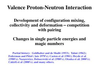
Valence Proton-Neutron Interaction. Development of configuration mixing, collectivity and deformation – competition with pairing Changes in single particle energies and magic numbers

Valence Proton-Neutron Interaction
E N D
Presentation Transcript
Valence Proton-Neutron Interaction Development of configuration mixing, collectivity and deformation – competition with pairing Changes in single particle energies and magic numbers Partial history: Goldhaber and de Shalit (1953); Talmi (1962); Federman and Pittel ( late 1970’s); Casten et al (1981); Heyde et al (1980’s); Nazarewicz, Dobacewski et al (1980’s); Otsuka et al( 2000’s); Cakirli et al (2000’s); and many others.
Measurements of p-n Interaction Strengths dVpn Average p-n interaction between last protons and last neutrons Double Difference of Binding Energies Vpn (Z,N) = ¼ [ {B(Z,N) - B(Z, N-2)} - {B(Z-2, N) - B(Z-2, N-2)} ] Ref: J.-y. Zhang and J. D. Garrett
Valence p-n interaction: Can we measure it? Vpn (Z,N) = ¼[ {B(Z,N) - B(Z, N-2)} - {B(Z-2, N) - B(Z-2, N-2)} ] - - - p n p n p n p n - Int. of last two n with Z protons, N-2 neutrons and with each other Int. of last two n with Z-2 protons, N-2 neutrons and with each other Empirical average interaction of last two neutrons with last two protons
Empirical interactions of the last proton with the last neutron Vpn (Z, N) = ¼{[B(Z, N ) – B(Z, N - 2)] - [B(Z - 2, N) – B(Z - 2, N -2)]}
Proton-neutron Interaction Strengths <p|V|n> = 1/ [ dn + dl + 1 ]
82 50 82 126 Orbit dependence of p-n interactions – simple ideas Low j, high n High j, low n
Z 82 , N < 126 Z 82 , N < 126 3 1 1 2 3 2 1 82 50 82 126 Z > 82 , N < 126 Z > 82 , N > 126
208Hg 208Hg
126 82 LOW j, HIGH n HIGH j, LOW n 50 82 Away from closed shells, these simple arguments are too crude. But some general predictions can be made p-n interaction is short range similar orbits give largest p-n interaction Largest p-n interactions if proton and neutron shells have similar fractional filling
82 50 82 126 Empirical p-n interaction strengths indeed strongest along diagonal. Empirical p-n interaction strengths stronger in like regions than unlike regions. Low j, high n High j, low n New mass data on Xe isotopes at ISOLTRAP – ISOLDE CERN Neidherr et al, preliminary
p-n interactions and the evolution of structure Direct correlation of observed growth rates of collectivity with empirical p-n interaction strengths
W. Nazarewicz, M. Stoitsov, W. Satula Realistic Calculations Microscopic Density Functional Calculations with Skyrme forces and different treatments of pairing
Agreement is remarkable. Especially so since these DFT calculations reproduce known masses only to ~ 1 MeV – yet the double difference embodied in dVpn allows one to focus on sensitive aspects of the wave functions that reflect specific correlations
Sensitivity of the mass filter:DFT with different pairing interactions
The new Xe mass measurements at ISOLDE give a new test of the DFT
dVpn (DFT – Two interactions) SLY4MIX SKPDMIX
Martin’s model (Sn, Te, Cd, Xe, Pd) dVpn = A +BS{1/ [ dnik + dlik + 1 ]} Vi2 Vk2 Sum is over all pairs of the i-th proton and k-th neutron orbits near the Fermi surface, as seen in the neighboring odd N and Z nuclei (in practice, levels up to ~ 300 keV). Parameters are A, B and D, the pairing gap parameter - chosen once for all the nuclei. Interestingly, the p-n interaction strength also depends on pairing! Might expect this simple, no-collective-correlations, model to work for Sn but not much else (because R4/2 >2 for Te, Cd, Xe, Pd).
One last thing Neidherr et al, preliminary Two regions of parabolic anomalies. Two regions of octupole correlations. Possible signature?
Summary of p-n interactions and dVpn p-n interactions and the evolution of collectivity Mass filters –dVpn– available far from stability Crossing pattern around doubly magic nuclei -- orbit overlaps Maximum for similar shell filling – along diagonal in N-Z plot Maximum in like quadrants (p-p or h-h vs p-h or h-p) Correlation with growth rates of collectivity Comparison with DFT calculations Possible signature of octupole correlations
How to know what the nuclei are telling us(using simple observables) • R4/2, but you all know that already, right? • Note: nuclear shapes have TWO variables so generally need TWO observables. • How shapes change with N and Z: P-factor • Bubbles and shell structure (already discussed) • How shapes change with N and Z: AHV model • How shapes change with spin – E-GOS • IBA (Its really simple, don’t be scared)
How does R4/2 vary and why do we care • We care because it is the only observable whose value immediately tells us something (not everything !!!) about the structure. • We care because it is easy to measure, especially far from stability • Other observables, like E(2+) and masses, are measurable even further from stability. They can give valuable information in the context of regional behavior.
Rotor E(I) (ħ2/2I )I(I+1) R4/2= 3.33 Doubly magic plus 2 nucleons R4/2< 2.0 Vibrator (H.O.) E(I) = n (0 ) R4/2= 2.0 8+. . . 6+. . . n = 2 n = 1 2+ n = 0 0+
Guide to R42 values in Collective Nuclei(R42 < 2 near closed shells) Axial Asym. R42~2.2 E(02) > E(2g) Def. Sph. E(02) < E(2g) Axial Sym. R42~2.9
Quantum phase transitions as a function of proton and neutron number Rotor Transitional Vibrator
Competition between pairing and the p-n interactions A simple microscopic guide to the evolution of structure (The next slides allow you to estimate the structure of any nucleus by multiplying and dividing two numbers each less than 30) (or, if you prefer, you can get the same result from 10 hours of supercomputer time)
NpNn p – n = P Np + Nn pairing p-n / pairing p-n interactions per pairing interaction Pairing int. ~ 1 MeV, p-n ~ 200 keV Hence takes ~ 5 p-n int. to compete with one pairing int. P ~ 5 P~5
Simple ways to see underlying shell structure Mid-sh. magic Onset of deformation as a phase transition mediated by a change in shell structure Onset of deformation “Crossing” and “Bubble” plots as indicators of phase transitional regions mediated by sub-shell changes
Often, esp. in exotic nuclei, R4/2 is not available. E(21+) [as 1/ E(21+) ], is easier to measure, works as well !!!
Two very useful techniques:Anharmonic Vibrator model (AHV)(works even for nuclei very far from vibrator)E-GOS Plots(Paddy Regan, inventor)
Anharmonic VibratorVery general tool, BOTH for yrast states and structural evolution R4/2 not exactly 2.0 in vibrational nuclei. Typ. ~2.2–ish. Write: E(4) = 2 E(2) + e where e is a phonon - phonon interaction. How many interactions in the 3 – phonon 6+ state? Answer: 3 How many in the n – phonon J = 2n state? Answer: n(n-1)/2 Hence we can write, in general, for the any “band”: E(J) = n E(2) + [n(n – 1)/2] e n = J/2 General. E.g., pure rotor, E(4) = 3.33E(2), hence e = 1.33 E(2) e /E(2) varies from 0 for harmonic vibrator to 1.33 for rotor !!!
E-GOS PlotsEGamma Over Spin Plot gamma ray energies going up a “band” divided by the spin of the initial state E-Gos plots are, for spin, what AHV plots are for N or Z Evolution of structure with J, N, or Z
E-GOS plots in limiting cases • Vibrator: E(I) = hw (I/2) • Hence Eg (I) = hw • Rotor: E(I) = h2/2J [I (I + 1)] • Hence Eg(I) = h2/2J [4I - 2] • AHV (R4/2 = 3.0): • E(4) = 2E(2) + e = 2E(2) + E(2) E(I) • = (I/2)E(2) + [(I/2) (I/2 -1)/2]E(2) • = (I/2)2 E(2) • Hence Eg(I) = 2(I + 2) R = 2 = constant
Comparisons of AHV and E-GOS with data J = 2 4 6 8 10 12 14 98-Ru 652 1397 2222 3126 4001 4912 5819 Egamma 652 745 825 904 875 911 907 AHV 652 1397 2235 3166 4190 5307 6517 (e = 93) e /E(2) = 0.14 E-GOS 326 189 137 113 87.5 76 64.8 ---------------------------------------------------------------------------------------------------------------- 166-Dy 77 253 527 892 1341 1868 2467 Egamma 77 176 274 365 449 527 599 AHV 77 253 528 902 1375 1947 2618 (e = 99) e /E(2) = 1.29 E-GOS 38 44 46 46 45 44 42.8
R4/2 = 3.0 (AHV) Vibr rotor
8+ 6+ 4+ 2+ 0+ Rotational states built on (superposed on) vibrational modes Vibrational excitations Rotational states
Why do the energies of rotational states differ from the rotor model??[You can see this by comparing with the rotor formula E ~ J ( J + 1). You can also see it deviations of E-GOS plots from the rotor expression, or with the AHV.] Look at the rotor formula: E(J) = [h2 /2I] x [ J ( J = 1)] where I is the moment of inertia. I is linear in BETA, the quadrupole deformation. There is a centrifugal force. If the potential in beta is SOFT, the nucleus can stretch, and beta will increase, so I will increase, so the energies will Decrease relative to the rotor expression with fixed I.
What to do with very sparse data??? Example: 190 W. How do we figure out its structure?
W-Isotopes N = 116