Hypothesis Testing
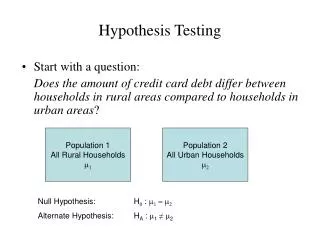
Hypothesis Testing. Start with a question: Does the amount of credit card debt differ between households in rural areas compared to households in urban areas ?. Population 1 All Rural Households m 1. Population 2 All Urban Households m 2. Null Hypothesis: H 0 : m 1 = m 2

Hypothesis Testing
E N D
Presentation Transcript
Hypothesis Testing • Start with a question: Does the amount of credit card debt differ between households in rural areas compared to households in urban areas? Population 1 All Rural Households m1 Population 2 All Urban Households m2 Null Hypothesis: H0 : m1 = m2 Alternate Hypothesis: HA : m1≠ m2
Take Random Sample (n2) Population 1 All Rural Households m1 Population 2 All Urban Households m2 Collect Data to Test Hypothesis Take Random Sample (n1) Are the sample means consistent with H0?
Summary Data Summary Rural Summary Urban Difference in means = $735 How likely is it to get a difference of $735 or greater if Ho is true? This probability is called the p-value. If small then reject Ho.
P-Value The probability of observing a difference between sample means as or more extreme as that observed if the null hypothesis is true. When this probability is small we declare that the two population means are significantly different. P< 0.05 is conventional cutoff Note: P-value and significance level are the same
test statistic: Computing P-Value for Testing Differences Between 2 Means Point estimator for m1-m2 Variability in point estimate Under Ho t follows a t-distribution with n1+ n2 -2 degrees of freedom (DF) Sp is pooled standard deviation, a weighted average of SD for each group
Observations • If Ho is true then t-values should center around 0 • A large difference between sample means will lead to a large t-value • A small standard error will lead to a large t-value • results from large sample sizes (n1 and n2) • results from small variation in the population
Assumptions for T-Test • Each of 2 populations follow a normal distribution • Data sampled independently from each population • Example of lack of independence Measure visual acuity in left and right eye • The population variances are the same for each population. The t-test is “robust” to violation of assumptions 1 and 3. Robust – the assumptions do not need to hold exactly
* SAS CODE FOR CREDIT CARD EXAMPLE; DATA credit; INFILE DATALINES; INPUT balance live @@; DATALINES; 9619 1 5364 1 8348 1 7348 1 381 1 2998 1 1686 1 1962 1 4920 1 5047 1 6644 1 7644 1 11169 1 7979 1 3258 1 8660 1 7511 1 14442 1 4447 1 6550 1 7581 2 12545 2 7959 2 2563 2 6787 2 5071 2 9536 2 4459 2 8047 2 8083 2 2153 2 8003 2 6795 2 5915 2 7164 2 9980 2 8718 2 8452 2 4935 2 5938 2 ; Used when inputing more than one obs per line
PROCMEANSDATA=credit ; CLASS live; VAR balance; The MEANS Procedure Analysis Variable : balance N live Obs N Mean Std Dev Minimum Maximum 1 20 20 6298.85 3412.31 381.0000000 14442.00 2 20 20 7034.20 2467.36 2153.00 12545.00
PROCTTESTDATA=credit ; CLASS live; VAR balance; OUTPUT The TTEST Procedure Statistics Lower CL Upper CL Lower CL Variable live N Mean Mean Mean Std Dev Std Dev balance 1 20 4701.8 6298.9 7895.9 2595 3412.3 balance 2 20 5879.4 7034.2 8189 1876.4 2467.4 balance Diff (1-2) -2641 -735.3 1170.8 2433.4 2977.6 Means for each group and the difference
PROCTTESTDATA=credit ; CLASS live; VAR balance; OUTPUT T-Tests Variable Method Variances DF t Value Pr > |t| balance Pooled Equal 38 -0.78 0.4397 balance Satterthwaite Unequal 34.6 -0.78 0.4401 T-statistic and P-value DF = n1+n2 – 2 Conclusion: Means are not significantly different (p=.44)
PROCTTESTDATA=credit ; CLASS live; VAR balance; OUTPUT Equality of Variances Variable Method Num DF Den DF F Value Pr > F balance Folded F 19 19 1.91 0.1666 Tests if variances are different between groups
Your Turn • Page 256 of Le • Compares cotinine levels from 8 infants from parents who smoke and 7 infants from parents who do not smoke. • What are the 2 populations? • Write down in words and symbols the null and alternate hypothesis • Write and run the SAS code to perform the t-test • Compare the SAS output with the calculations on page 256 • What is the p-value for the test?
Matched Pair Data • Each subject serves as own control • Half of patients start out on treatment 1, other half on treatment 2 • Outcome is measured at end of first period • Patients are switched to other treatment (usually after a “washout” period). • Outcome is measured at end of second period • Analyses is based on within subject differences
Matched Pair Data Examples • Data on twins • Pre-post tests • Data on pairs of eyes, left versus right foot, etc
Matched Pair Data • Analyses reduced to a 1-sample problem • Differences are computed for each pair • di = outcome when on treatment 1 minus outcome when on treatment 2 Large values indicate differences in treatments
Matched Pair Example • Question: Does intake of oat bran lower your cholesterol? • LDL cholesterol measured on 14 subjects • After period on cornflake diet • After period on oat bran diet • Data on page 273 of Le
DATA oatbran; INFILE DATALINES; INPUT subject $ cornflakes oatbran ; oatcorndif = oatbran - cornflakes; DATALINES; 1 4.61 3.84 2 6.42 5.57 3 5.40 5.85 4 4.54 4.80 5 3.98 3.68 6 3.82 2.96 7 5.01 4.41 8 4.34 3.72 9 3.80 3.49 10 4.56 3.84 11 5.35 5.26 12 3.89 3.73 13 2.25 1.84 14 4.24 4.14 ;
*Running Matched Pair T-test • using proc means: ; • PROC MEANSDATA=oatbran NMEANSTDERRT PRT ; • VAR oatcorndif OUTPUT The MEANS Procedure Variable N Mean Std Error t Value Pr > |t| ƒƒƒƒƒƒƒƒƒƒƒƒƒƒƒƒƒƒƒƒƒƒƒƒƒƒƒƒƒƒƒƒƒƒƒƒƒƒƒƒƒƒƒƒƒƒƒƒƒƒƒƒƒƒƒƒƒƒƒƒƒƒƒƒƒƒƒƒƒƒƒ cornflakes 14 4.4435714 0.2589319 17.16 <.0001 oatbran 14 4.0807143 0.2824898 14.45 <.0001 oatcorndif 14 -0.3628571 0.1084984 -3.34 0.0053 Tvalue = mean/se Conclusion: Oat bran significantly reduces cholesterol (p<.01)
*Running Matched Pair T-test using PROC TTEST; PROCTTEST; VAR oatcorndif; RUN; No class variable so performing one sample t-test. Tests if mean is 0.
Match Pair Data- Your Turn Female killdeer lay four eggs each spring. A scientist claims that the egg that hatches first yields a larger bird than the one that hatches last. To test his claim, he weighs the oldest and youngest of eight families with the following results: Test the researcher’s hypothesis using the data above? What is the null and alternative hypothesis? What is the p-value for the test?
Issues with hypothesis testing • Significance does not imply causality • Need a proper prospective experiment • Significance does not imply practical importance • Trivial but significant differences • Run lots of tests, will find significant difference by chance • With α = 0.05, expect 1 in 20 results to be sig. by chance
Issues with hypothesis testing • Large p-values because sample size is small • Effect could exist but we may not have a large enough sample size • Outliers may cause problems
Issues With Hypothesis Testing What is the population of inference? Example: A statistics class of n=15 women and n=5 men yield the following exam scores: Women: mean = 90% SD = 10% Men: mean = 85% SD = 11% Test the hypothesis that women did better on the exam then men.

