Stereo matching Class 10
Stereo matching Class 10. Read Chapter 7 http://cat.middlebury.edu/stereo/. Tsukuba dataset. Stereo. Standard stereo geometry Stereo matching Correlation Optimization (DP, GC) General camera configuration Rectification Plane-sweep. Standard stereo geometry.


Stereo matching Class 10
E N D
Presentation Transcript
Stereo matchingClass 10 Read Chapter 7 http://cat.middlebury.edu/stereo/ Tsukuba dataset
Stereo • Standard stereo geometry • Stereo matching • Correlation • Optimization (DP, GC) • General camera configuration • Rectification • Plane-sweep
Standard stereo geometry pure translation along X-axis
Stereo matching • Search is limited to epipolar line (1D) • Look for most similar pixel ?
Aggregation • Use more than one pixel • Assume neighbors have similar disparities* • Use correlation window containing pixel • Allows to use SSD, ZNCC, Census, etc.
Comparing image regions Compare intensities pixel-by-pixel I(x,y) I´(x,y) Dissimilarity measures • Sum of Square Differences
Comparing image regions Compare intensities pixel-by-pixel I(x,y) I´(x,y) Similarity measures Zero-mean Normalized Cross Correlation
Comparing image regions Compare intensities pixel-by-pixel I(x,y) I´(x,y) Similarity measures Census only compare bit signature (Real-time chip from TYZX based on Census)
Small windows disparities similar more ambiguities accurate when correct Large windows larger disp. variation more discriminant often more robust use shiftable windows to deal with discontinuities Aggregation window sizes (Illustration from Pascal Fua)
Occlusions (Slide from Pascal Fua)
Real-time stereo on GPU (Yang and Pollefeys, CVPR2003) • Computes Sum-of-Square-Differences (use pixelshader) • Hardware mip-map generation for aggregation over window • Trade-off between small and large support window 290M disparity hypothesis/sec (Radeon9800pro) e.g. 512x512x36disparities at 30Hz GPU is great for vision too!
Ordering constraint surface slice surface as a path 6 5 occlusion left 4 3 2 1 4,5 6 1 2,3 5 6 2,3 4 occlusion right 1 3 6 1 2 4,5
Uniqueness constraint • In an image pair each pixel has at most one corresponding pixel • In general one corresponding pixel • In case of occlusion there is none
use reconstructed features to determine bounding box Disparity constraint surface slice surface as a path bounding box disparity band constant disparity surfaces
Similarity measure (SSD or NCC) Optimal path (dynamic programming ) Stereo matching • Constraints • epipolar • ordering • uniqueness • disparity limit • Trade-off • Matching cost (data) • Discontinuities (prior) Consider all paths that satisfy the constraints pick best using dynamic programming
Hierarchical stereo matching Allows faster computation Deals with large disparity ranges Downsampling (Gaussian pyramid) Disparity propagation
Disparity map image I´(x´,y´) image I(x,y) Disparity map D(x,y) (x´,y´)=(x+D(x,y),y)
Energy minimization (Slide from Pascal Fua)
Graph Cut (general formulation requires multi-way cut!) (Slide from Pascal Fua)
Simplified graph cut (Roy and Cox ICCV‘98) (Boykov et al ICCV‘99)
~ image size (calibrated) Planar rectification Distortion minimization (uncalibrated) Bring two views to standard stereo setup (moves epipole to ) (not possible when in/close to image)
Polar rectification (Pollefeys et al. ICCV’99) Polar re-parameterization around epipoles Requires only (oriented) epipolar geometry Preserve length of epipolar lines Choose so that no pixels are compressed original image rectified image Works for all relative motions Guarantees minimal image size
original image pair planar rectification polar rectification
Example: Béguinage of Leuven Does not work with standard Homography-based approaches
Stereo camera configurations (Slide from Pascal Fua)
Multi-camera configurations (illustration from Pascal Fua) Okutami and Kanade
Multi-view depth fusion (Koch, Pollefeys and Van Gool. ECCV‘98) • Compute depth for every pixel of reference image • Triangulation • Use multiple views • Up- and down sequence • Use Kalman filter Allows to compute robust texture
Plane-sweep multi-view matching • Simple algorithm for multiple cameras • no rectification necessary • doesn’t deal with occlusions Collins’96; Roy and Cox’98 (GC); Yang et al.’02/’03 (GPU)