Data Process
Spring Semester 2005 Experimental Method and Data Process. Data Process. Kihyeon Cho Kyungpook National University. Contents. High Energy Physics Data Processing Fitting Conclusions. High Energy Physics. Goal.

Data Process
E N D
Presentation Transcript
Spring Semester 2005Experimental Method and Data Process Data Process Kihyeon Cho Kyungpook National University
Contents • High Energy Physics • Data Processing • Fitting • Conclusions
Goal The ultimate structure of matter and the understanding of the origin of universe High Energy Physics Direction
What is World Made of? • Atom • Electron • Nucleus • Proton, neutron • quarks (100 pm) (1 fm) (1 am)
How do we experiment with tiny particles? (Accelerators) • Accelerators solve two problems: • High energy gives small wavelength to detect small particles. • The high energy create the massive particles that the physicist want to study.
World-wide High Energy Physics Experiment • Europe • In 2007, the LHC will be completed at CERN • Two big experiments (ATLAS, CMS) in collab. of HEP institutes and physicists all over the world • CERN, IN2P3(France), and INFN(Italy) are preparing HEP Grid for it. • USA • The BaBar Exp at SLAC • The Run II of the Tevatron at Fermilab (CDF and D0) • The CLEO at Cornell • The LHC experiments at CERN (ATLAS, CMS) • The RHIC exp at BNL • The Super-K in Japan • The HEP Grid in the ESNET program • Japan • Belle at KEK • Super-K, Kamioka • LHC at CERN (ATLAS) • The RHIC at BNL (USA) • They are now working for it. Global Collaboration • Korea • We have most of these world-wide experimental programs…
연구내용 GermanyDESY Space Station (ISS) US FNAL ChinaIHEP USBNL EuropeCERN Korea CHEP JapanKEK
Where is Fermilab? • 20 mile west of Chicago • U.S.A Fermilab
Booster p source Main Injector and Recycler Overview of Fermilab CDF Fixed Target Experiment D0
Fermi National Accelerator Laboratory Highest Energy Accelerator in the World Energy Frontier: CDF, D0 Search for New Physics (Higgs, SUSY, quark composites,… Precision Frontier: charm, kaon, neutrino physics (FOCUS, KTeV, NUMI/MINOS,BOONE,…etc. Connection to Cosmology: Sloan Digital sky survey, Pierre Auger,… Largest HEP Laboratory in USA 2200 employees 2300 users (researchers from univ.) Budget is >$300 million
Why do we do experiments? • Parameter determination • To set the numerical values of some physical quantities • Ex) To measure velocity of light • Hypothesis testing • To test whether a particular theory is consistent with our data • Ex) To check whether velocity of light has suddenly increased by several percent since beginning of this year
Type of Data • Real Data (on-site) • Raw Data : Detector Information • Reconstructed Data : Physics Information • Stream (Skim) Data : Selected interested physics • Simulated Data (on-site or off-site) • Physics generation : pythia, QQ, bgenerator, CompHEP, … • Detector Simulation : Fastsim, GEANT, …
Research Method Remote-sites (CHEP + participating institutions) Data Analysis HEP Knowledge Reaction Simulation = Event Generation Detector Simulation Simulated Data Data Reduction Real Data On-sites (Experimental sites)
Error () • Error • Error : the difference between measurement and true value • True value • We don’t know it • Statistical error • Error due to statistical fluctuation • Systematic error • More in nature of mistakes due to equipments and experimentalists • Experimental value : Meas. stat. error sys. error Example ) m(top) = 175.9 4.8 5.3 GeV/c2 (CDF, 1998)
Why estimate errors? • To know how accuracy of the measurement • Example • The conventional speed of light c=2.998 X 10⁸ m/sec • When the new measurement c=3.09 X 10⁸ m/sec • Case 1. If the error is 0.15, then it is consistent. • Conventional physics is in good shape. • 3.09 0.15 is consistent with 2.998 X 10⁸ m/sec • Case 2 . If the error is 0.01, then it is not consistent. • 3.09 0.01 is world shattering discovery. • Case 3. If the error is 2, then it is consistent. • However, the accuracy of 3.09 2 is too low. • Useless measurement Whenever you determine a parameter, estimate the error or your experiment is useless.
Examples) Bad and Good Bad Good
How to reduce errors? • Statistical error • Repeated measurement • N : the expected number of observation • = Sqrt(N) : the spread • Systematic error • No exact formulae • Ideal case : All such effects should be absent. • Real world : An attempt to be made to reduce it.
How to solve systematic errors? • Use constraint condition • Ex) Triangle • Calibrations • Energy and momentum conservation • E(after) – E(before) = 0 • |P(after)| - |P(before)| = 0 How small of the systematic error? • Systematic errors should be around statistical errors
The meaning of (error) • Distributions x -> n(x) • Discrete • ex) # of times n(x) you met a girl at age x • Continuous : • ex) Hours sleep each night (x), # of people sleeping for time. For an even larger number of observation and with small bin size, the histogram approach a continuous distribution. • Mean and Variance • Gaussian distribution • In case of larger number of observation • It is important for error calculations
Ksp+p- Tracking Performance Hit Resolution ~200mm Goal : 180mm Residual distance (cm) COT tracks L p-p
Mean and Variance In fact, we don’t know the true value in the real world.
Mean • Mean • N events has the value of (x1, x2, x3,… xN) • Median – Observation or potential observation in a set that divides the set so that the same number of values, it is the middle value; for an even number it is the average of the middle tow • Mode – Observation that occurs with the greatest frequency • When do not know true value
Variance • Variance • When know true value • When do not know true value
Accuracy () • In order to know the accuracy of the measurement
Gaussian Distribution • In case of large size of data • Gaussian distribution is the fundamental in error treatment.
Gaussian Distribution (cont’d) • The normalized function • Mean () • Width () • Width () is smaller, distribution is narrower. • Properties
Gaussian Distribution (cont’d) • Mean () is same as zero. • However width ( ) is different.
Examples (Gaussian + BG) D.J.Kong (2004.3.4)
CDF Secondary Vertex Trigger NEW for Run 2 -- level 2 impact parameter trigger Provides access to hadronic B decays Data from commissioning run COT defines track SVX measures (no alignment or calibrations) at level 1 impact parameter s ~ 87 mm d (cm)
Gaussian fitting Using Mn_fit - +
Significant Figure • The measured value has meaning by significant figures • Significant Figure • It includes the first figure of uncertainty • All the figures between LSD (least significant digit) and MSD(Most significant digit) • LSD • If there is no point : The far right non-zero figure ex)23000 • If there is point : The far right figure ex) 0.2300 • MSD : The far left non-zero figure
Significant Figure (Example) • 4 digit : 1234, 123400, 123.4, 1000. • 4 digit : 10.10, 0.0001010, 100.0, 1.010X10³ • 3 digit : 1010 cf) 1010. (Four digit of significant figure)
The calculation • Add and Subtract • The last result is decided by the minimum point of calculations • Example) 123 + 5.35 -------- 128.35 1.0001 ( 5 digit of SF) + 0.0003 (1 digit of SF) -------- 1.0004 (5 digit of SF)
Calculations (cont’d) • Multiply and Divide • Same as the minimum digit of significant figure • Example) 16.3 X 4.5 = 73.35 => 73
Propagation of Errors • Suppose that (x1,x2, …) is the variables, then variation of the function of F(x1, x2, …) is as follows: • In case that there is no correlation between variables
Propagation of Errors (continued) • Suppose that (x1,x2, …) is the variables, then variation of the function of F(x1, x2, …) is as follows: - In case that there is correlation between variables Let us consider only non-correlation case.
Combining Errors • Add or Subtract (F=x1+x2 or F= x1-x2) Example) x1 =100. 10. + x2 = 400. 20. ----------- F = 500. 22. Example) The error of the measurement
Combining Errors (cont’d) • F=ax (a is constant) Example) x =100. 10. a = 5 ------------ F = 500. 50.
Combining Errors (cont’d) • Multiplication (F=x1•x2) Example) x1 =100. 10. x2 = 400. 20. ----------- F = (400. 45. ) X 102
Combining Errors (cont’d) • Division (F= x1/ x2) Example) x1 =100. 10. x2 = 400. 20. ----------- F = 0.250 0.028
Combining results Using weighting factor • Cases • With different detection efficiencies (RunI, RunII) • With different parts of apparatus (SVX, COT) • With different experiment (CDF, D0) • With different decay mechanisms ex) Bs->Psi(2s) Phi 1) Psi(2s) ->J/Psi mu+ mu- 2) Psi(2s) -> mu+mu- ex) D0-> KsKs 1) D*+ -> D0 pi+ 2) D*0 -> D0 pi0
Combining results Using weighting factor (cont’d) • Average • There is N data whose values are (x1, x2,. ..xk,… xN) • Suppose that the error of Xk is k where weighting factor • Error :