The Univariate AutoRegressive Model
190 likes | 222 Vues
The Univariate AutoRegressive Model. X t = [a 1 X t-1 + a 2 X t-2 + a 3 X t-3 + … + a m X t-m ] + ε t where X is a zero-mean stationary stochastic process, a i are model coefficients, m is the model order, and ε t is the white noise residual error process.

The Univariate AutoRegressive Model
E N D
Presentation Transcript
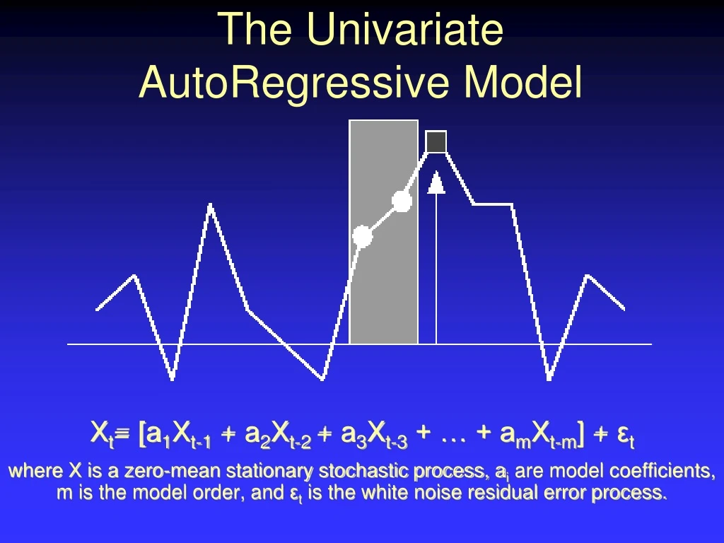
The UnivariateAutoRegressive Model Xt= [a1Xt-1 + a2Xt-2 + a3Xt-3 + … + amXt-m] + εt where X is a zero-mean stationary stochastic process, ai are model coefficients, m is the model order, and εt is the white noise residual error process.
The MultiVariate AutoRegressive (MVAR) Model Xi,t= ai,1,1X1,t-1 + ai,1,2X1,t-2 + … + ai,1,mX1,t-m + ai,2,1X2,t-1 + ai,2,2X2,t-2 + … + ai,2,mX2,t-m + … + ai,p,1Xp,t-1 + ai,p,2Xp,t-2 + … + ai,p,m Xp,t-m + ei,t Xt = A1Xt-1 + + AmXt-m + Et where: Xt = [x1t , x2t , , xpt ]T are p data channels, m is the model order, Ak are p x m coefficient matrices, & Et is the white noise residual error process vector.
MVAR Modeling ofEvent-Related Neural Time Series • Repeated trials are treated as realizations of a stationary stochastic process. • Ak are obtained by solving the multivariate Yule-Walker equations (of size mp2), using the Levinson, Wiggens, Robinson algorithm, as implemented by Morf et al. (1978). (Morf M, Vieira A, Lee D, Kailath T (1978) Recursive multichannel maximum entropy spectral estimation. IEEE Trans Geoscience Electronics 16: 85-94) • The model order is determined by parametric testing.
Spectral Analysis by MVAR Modeling • The Spectral Matrix is defined as: S( f ) = <X (f ) X (f )*> = H(f ) H*(f ) where * denotes matrix transposition & complex conjugation; is the covariance matrix of Et ; and is the transfer function of the system. • The Power Spectrum of channel k is Skk ( f ) which is the k th diagonal element of the spectral matrix.
Definitions Let Xk(f) and Xl(f) be the Fourier Transforms of Xk(t) and Xl(t). Cross-Power Spectrum: Auto-Power Spectra:
Cross-Spectral Analysis by MVAR Modeling • The Cross-Spectrum of channels k & l is Skl ( f ). • The (squared) Coherence Spectrum of channels k & l is the cross-power normalized by the two auto-powers: γkl ( f ) = Pkl ( f ) / Pkk ( f ) Pll ( f ). • The value of coherence at frequency f can range from 1, indicating maximum interdependence, down to 0, indicating no interdependence. The phase of the cross spectrum plotted as a function of f gives the phase spectrum.
Statistical Causality For two simultaneous time series, one series is called causal to the other if we can better predict the second series by incorporating knowledge of the first one (Wiener, The Theory of Prediction, 1956).
Granger Causality Granger (1969) implemented the idea of causality in terms of autoregressive models.Let x1, x2, …, xtand y1, y2, …, yt represent two time series. Granger compared two linear models: xt = a1xt-1+ … + amxt-m+t and xt = b1xt-1+ … + bmxt-m + c1yt-1+ … + cmyt-m+ t Restricted Model Unrestricted Model
Interpretation of Causal Influence If Then, in some suitable statistical sense, we can say that the y time series has a casual influence on the x time series.
Granger Causal Spectrum Geweke (1982) found a spectral representation of the time domain Granger causality:
Granger Causal Spectrum The Granger Causal Spectrum from y to x is: where ω is frequency in rads/sec,Sxx is the autospectrum of x, Hxx(ω) is an element of the transfer function H(ω)=A-1(ω), 2 is the residual variance of the unrestricted model of x, and * denotes complex conjugation and matrix transposition. The spectral Granger Causality is expressed as the natural log of the ratio of total power of x over intrinsic (non-causal) power. The causal influence is zero when the intrinsic power equals the total power, and the causal power is zero. The causal influence increases as the intrinsic power decreases, and the causal power increases.
Granger Causality Graph IT1 PST1 PST2 STR1 STR2 STR3
AMVAR Analysis of Neural Dynamics Adaptive MultiVariate AutoRegressive (AMVAR) modeling captures the dynamics of neural processes with a short time resolution, i.e. on the order of 50 msec. (Ding, Bressler et al., Biological Cybernetics, 2000)