Chapter 5: Linear Algebra Applications
220 likes | 687 Vues
Chapter 5: Linear Algebra Applications. Homogeneous Linear Equations Non-homogeneous equation Eigen v alue problem. 5.1 Homogeneous linear Equations. N=3; The problem is to solve : There is an obvious solution: But is it the only one?

Chapter 5: Linear Algebra Applications
E N D
Presentation Transcript
Chapter 5: Linear Algebra Applications Homogeneous Linear Equations Non-homogeneous equation Eigen valueproblem
5.1 Homogeneous linear Equations N=3; The problem is to solve : There is an obvious solution: But is it the only one? Consider the determinant By using the rules of determinants that we proved in chapter 4, we compute the following: But the left column is zero by assumption of our linear system of equations, and thus . And thus if our starting homogeneous equations are to be satisfied we need: and likewise we could just as easily have gotten: and . These equations are satisfied if x=y=z=0 (our obvious solution) but can also have a solution for non-zero (x,y,z)’s if det[a]=0 Conclusion: Non-zero solutions to homogeneous linear equations are possible only if the matrix of the coefficients of the equations has a zero determinant. 5.1. Solution to homogeneous linear equations.
5.1 Homogeneous linear Equations 5.1 Solution to homogeneous linear equations cont’d. E5.1-1 Consider the system of equations What are the possible solutions? If applicable, find the equation of the set of solutions. E5.1-2 Consider the system of equations What are the possible solutions? If applicable, find the equation of the set of solutions.
II. INHOMOGENEOUS EQN 5.2 Inhomogeneous Equations: Again for n=3 (but the generalization to any n is obvious) the problem is: In matrix form we have: where: and Assuming a non-zero determinant, we can use the inverse to solve for: and thus we get the solution for immediately by: In case the determinant of [a] is zero, the inverse of [a] does not exist. Since the determinant is zero, it means that the left hand sides of the equations are linearly dependent. For instance in our n=3 case above we could have: (1st row = * 2nd row) Then we have 2 possible cases: in which case the 2 proportional equations are consistent. and the system has an infinite number of solutions points. Since we have 3 unknowns (x,y,z) and only 2 independent equations the space of solution is a line (the intersection of 2 planes). Note; we could also have further dependence: say, the 3rd row is proportional to the second one. In that case there would be one independent equation (i.e. the 3 equations are proportional to each other) then the space of solutions would be would be a plane of equation, say, if equations 2 and 3 are consistent or, again, we have the possibility of no solutions if equations 2 and 3 are NOT consistent: for instance but E 5.2-1 : Consider the matrix Find and discuss solution(S) to E 5.2-2 : Consider the matrix Find and discuss solution(S) to
II. INHOMOGENEOUS EQN 5.2 Inhomogeneous Equations: E 5.2-3 : Consider the matrix Find and discuss solution(S) to
5.3 EIGENVALUE PROBLEM 5.3 Eigenvalue PROBLEM PROBLEM STATEMENT: Given a matrix A, the problem is to find out if there exist vectors V such that: [5.3-1] Such vectors are called eigenvectors associated with the eigen value Necessary Condition For The Existences Eigenvectors: If V exist then: [5.3-2] and thus: [5.3-3] 5.3-1 prove this using known matrix operation: add. and mult. of matrices and mult. of matrix by number From what we learned in 5.2, we know that in order to get a non-zero (i.e. =0) solution of [5.3-3], the determinant of matrix must be zero. Requiring the determinant to be zero we get: det This is called the characteristic equation. In n=3 this is a cubic equation in that will have at most three roots called the eigenvalues of the matrix. (for nxn determinants the char. Equation will have at most n eigenvalues.) For each eigenvalue we can find a corresponding eigenvector satisfying [5.3-1]. Note however that if is a eigenvector of the eigenvalue then so is the vector since . Thus if a vector is an eigenvector, then so will be all vectors proportional to it. NOTE: Some eigenvalues can be of higher multiplicity. For instance, if the characteristic equation has a factor of the form (…..) then appears as a an eigenvalue of multiplicity 2.
5.3 EIGENVALUE PROBLEM 5.3 Eigenvalue PROBLEM EXAMPLE: consider the matrix Lets compute e-values and e-vectors.
5.3 EIGENVALUE PROBLEM 5.3 Eigenvalue PROBLEM EXAMPLE: consider the matrix Lets compute e-values and e-vectors.
5.3 EIGENVALUE PROBLEM 5.3 Eigenvalue PROBLEM EXAMPLE: consider the matrix Lets compute e-values and e-vectors.
5.3 EIGENVALUE PROBLEM 5.3 Eigenvalue PROBLEM SOME PROPERTIES of EIGENVECTORS and EIGENVALUES: Theorem: Eigenvectors associated with distinct eigenvalues form a linearly independent set. Proof (by contradiction): Let’s do it for n=3 For simplicity. Assume the set is linearly dependent. Thus we can write: [5.3-4] Now let’s apply the matrix a on the equation: since the vi’s are e-vectors: Which implies that: and finally comparing this to [5.3-4] we conclude that and which contradicts our assumption that the e-values are different. And thus the vi’s cannot be linearly dependent. For eigenvalues of multiplicity s more than one (also called DEGENERATE eigenvalues), one can find at most s linearly independent eigenvectors. For matrices over complex numbers, the characteristic equations always n roots (although some could be degenerate. Notice that if =0 is an eigenvalue of a, then a is not invertible. Proof: since is an e-value then det and since =0, thus det (a) =0 as well; proving that a is not invertible.
5.3 EIGENVALUE PROBLEM 5.3 Eigenvalue PROBLEM: Diagonalization of matrices An nxn matrix A is said to be diagonalizable if there exist a matrix P such that A=PDP-1 (or equivalently P-1AP=D) where D is a diagonal matrix. Theorem: P exists if and only if there exist n independent eigenvectors of A; Consider the n independent eigenvectors of A: in that case P is made up of the eigenvectors of A, entered as column coefficients. D is in addition found to be made up of the corresponding eigenvalues of A Proof for n=3 (general case identical) Consider the 3 independent eigenvectors of A: Let’s compute AP (notice that the elements of P are the e-vectors components in COLUMN form): Since in an eigenvector, we know that: and thus if we look, for instance, at the x component we get: and likewise for the other components of v1 as well as the other vectors; for instance: This means that we can rewrite the above product of matrices as: E5.3-2 In the above is equal to which element of the matrix AP?
5.3 EIGENVALUE PROBLEM 5.3 Eigenvalue PROBLEM: Diagonalization of matrices Now let’s compute PD where D is the diagonal matrix of the eigenvalues arranged in the same order as their corresponding eigenvectors in the matrix P. We get: But that’s exactly the same answer as we got on the previous page computing AP!!! So we can conclude that: AP=PD and thus, if P is invertible (i.e. its det is non-zero and thus the eigenvector are linearly independent!), we finally obtain: A=PDP-1 where P is the matrix of the eigenvectors of A in column placement and D is the diagonal matrix of the eigenvalues of A is in the same position as the eigenvectors in P: If some of the eigenvalues are degenerate one can carry out the same procedure as long as one can find n linearly independent eigenvectors. In the next chapter we’ll look at a few examples of this procedure in concrete physical cases.
5.3 EIGENVALUE PROBLEM 5.3 Eigenvalue PROBLEM: Diagonalization of matrices Example of diagonalization of A=
5.3 EIGENVALUE PROBLEM 5.3 Eigenvalue PROBLEM: Diagonalization of matrices Example of diagonalization of A=
5.3 EIGENVALUE PROBLEM 5.3 Eigenvalue PROBLEM E5.3-3 Consider the matrix: Find the characteristic equations, eigenvalues and eigenvectors (normalized). Explain whether or not the matrix can be diagonalized, considering the eigen vectors. If it can, continue and find matrices P and D and verify that P does indeed diagonalize A. E5.3-4 Repeat above steps for and then check with mathematica eigenvalues and eigenvectors. E5.3-5 Consider the matrix of a 30 degree counterclockwise rotation in 2 dimensions. Can you find real eigenvalues/ eigenvectors? Comment on your result as it pertains to the diagonalization of a rotation matrix. E5.3-6 Take an 4x4 matrix of your choice. Compute its eigenvectors and eigenvalues using mathematica. Still using mathematica compute P-1AP and verify that you indeed get the diagonal matrix of its corresponding eigenvalues. If the matrix yu found is not diagonalizable choose a different one and repeat calculation
![linear algebra - chapter 1 [yr2005]](https://cdn4.slideserve.com/146212/slide1-dt.jpg)