Download
1 / 14
160 likes | 238 Vues
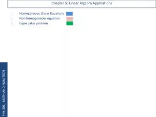
Dive into linear algebra applications using Matlab functions for matrix operations such as dot, cross products. Learn how to solve linear equations with Gaussian elimination, handle singular matrices, and explore the concept of rank.

E N D
ME 303 Linear Algebra Applications in Matlab
Some Matrix Operations The dot operator. plays a specific role in MATLAB. It is used for the componentwise applicationof the operator that follows the dot operator After this point a=a’
Some Matrix Operations • The cross product of two three-dimensional vectors is calculated using command cross. Let thevector a be the same as above and let • This creates a 3-by-3 matrix To delete a row (column) use the empty vector operator [ ]
Some Matrix Operations • Second column of the matrix A is now deleted. To insert a row (column) we use the technique forcreating matrices and vectors Using MATLAB commands one can easily extract those entries of a matrix that Satisfyan impsedcondition.
Special Matrices • There are several special matrices which deserve some attention. The first is the diagonalmatrix, which is a matrix whose only non-zero elements lie along the matrix diagonal, i.e.the elements for which the row and column indices are equal. Another special matrix of interest is the identity matrix, typically denoted as I. The identitymatrix is always square (number of rows equals number of columns) and contains ones onthe diagonal and zeros everywhere else.
Solving Systems of Linear Equations • MATLAB has several tool needed for computing a solution of the system of linear equations. • Let Xbe an m-by-n matrix and let b be an m-dimensional (column) vector. To solvethe linear system Xb = yone can use the backslash operator \ , which is also called the leftdivision. • Consider the followingsystem of 3 equations in 3 unknowns
Gaussian Elimination • The problem is to find the values of b1, b2 and b3 that make the system of equations hold.To do this, we can apply Gaussian elimination. This process starts by subtracting amultiple of the first equation from the remaining equations so that b1 is eliminated fromthem. • We see here that subtracting 2 times the first equation from the second equationshould eliminate b1. Similarly, subtracting -2 times the first equation from the thirdequation will again eliminate b1. The result after these first two operations is: The first coefficient in the first equation, the 2, is known as the pivot in the first eliminationstep. We continue the process by eliminating b2 in all equations after the second, which inthis case is just the third equation. This is done by subtracting 4 times the second equationfrom the third equation to produce:
Gaussian Elimination • In this step the 1, the second coefficient in the second equation, was the pivot. We havenow created an upper triangular matrix, one where all elements below the main diagonal arezero. This system can now be easily solved by back-substitution. It is apparent from thelast equation that b3 = 1. Substituting this into the second equation yields b2 = -2.Substituting b3 = 1 and b2 = -2 into the first equation we find that b1 = 1. • Gaussian elimination is done in MATLAB with the left division operator \ (for moreinformation about \ type help mldivide at the command line). Our example problemcan be easily solved as follows: It is easy to see how this algorithm can be extended to a system of n equation in n Unknowns!!!
Singular Matrices and the Concept of Rank • Gaussian elimination appears straightforward enough, however, are there some conditionsunder which the algorithm may break down? • It turns out that, yes, there are. Some of theseconditions are easily fixed while others are more serious. • The most common problemoccurs when one of the pivots is found to be zero. If this is the case, the coefficients belowthe pivot cannot be eliminated by subtracting a multiple of the pivot equation. • Sometimesthis is easily fixed: an equation from below the pivot equation with a non-zero coefficient inthe pivot column can be swapped with the pivot equation and elimination can proceed. • However, if all of the coefficients below the zero pivot are also zero, elimination cannotproceed. • In this case, the matrix is called singular and there is no hope for a unique solutionto the problem. • As an example, consider the following system of equations:
Singular Matrices and the Concept of Rank • Elementary row operations can be used to produce the system: This system has no solution as the second equation requires that b3 = 1/3 while the thirdequation requires that b3 = -2. If we tried this problem in MATLAB we would see thefollowing:
Singular Matrices and the Concept of Rank • On the other hand, if the right hand side of the system were changed so that we startedwith: This would be reduced by elementary row operations to: Note that the final two equations have the same solution, b3 = -2. Substitution of this resultinto the first equation yields b1 + 2b2 = 3, which has infinitely many solutions. We can seethat singular matrices can cause us to have no solution or infinitely many solutions.
Singular Matrices and the Concept of Rank If wedo this problem in MATLAB we obtain: The solution obtained agrees with the one we calculated above, i.e. b3 = -2. From theinfinite number of possible solutions for b1 and b2 MATLAB chose the values -14.3333and 8.6667, respectively.