Outline
Outline. Quantum Braitenberg Vehicles Programmable Braitenberg Vehicles Combinational and Quantum Circuits Deterministic, Probabilistic, and Entangled Behaviors Examples or our Robots Quantum Search Quantum Emotional Robots Curriculum Research. Part 2:. Quantum Search.

Outline
E N D
Presentation Transcript
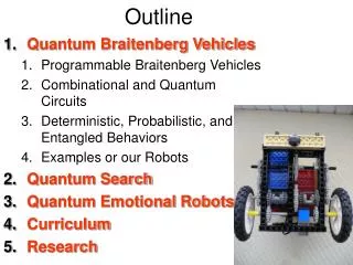
Outline • Quantum Braitenberg Vehicles • Programmable Braitenberg Vehicles • Combinational and Quantum Circuits • Deterministic, Probabilistic, and Entangled Behaviors • Examples or our Robots • Quantum Search • Quantum Emotional Robots • Curriculum • Research
Part 2: Quantum Search
Graph Coloring • Building oracle for graph coloring is a better explanation of Grover than database search. • This is not an optimal way to do graph coloring but explains well the principle of building oracles. The Graph Coloring Problem 1 Color every node with a color. Every two nodes that share an edge should have different colors. Number of colors should be minimum 1 3 2 3 2 5 4 5 4 6 7 6 7 This graph is 3-colorable
Simpler Graph Coloring Problem 1 3 2 We need to give all possible colors here 4 Two wires for color of node 1 Two wires for color of node 2 Two wires for color of node 3 Two wires for color of node 4 Gives “1” when nodes 1 and 2 have different colors 13 23 24 34 12 F(x) Value 1 for good coloring
Simpler Graph Coloring Problem We need to give all possible colors here Give Hadamard for each wire to get superposition of all state, which means the set of all colorings H |0> |0> H |0> H H H 13 23 24 34 12 Discuss naïve non-quantum circuit with a full counter of minterms f(x) Value 1 for good coloring Now we will generate whole Kmap at once using quantum properties - Hadamard
Simplified schematic of our Graph Coloring Oracle. “Classical” Quantum Computer Circuit Model for Graph Coloring We designed 35 oracles
Hadamard Transform Single qubit H = H H = 1/2 Parallel connection of two Hadamard gates is calculated by Kronecker Product (tensor product) Here I calculated Kronecker product of two Hadamards
Motivating calculations for 3 variables |0> H |0> + |1> |1> H |0> - |1> • As we remember, these are transformations of Hadamard gate: In general: |x> H |0> + (-1) x |1> For 3 bits, vector of 3 Hadamards works as follows: From multiplication |abc> (|0>+(-1)a|1>) (|0>+(-1)b|1>) (|0>+(-1)c|1>) = |000> +(-1)c |001> +(-1)b |001>+(-1)b+c |001>000> +(-1)a |001> + (-1)a+c |001> + (-1)a+b |001> (-1)a+b+c |001> If a = b = c =0 then all phases positive
|0> oracle |000> +|001> + |010>+|011> +|100> + |101> +|110> + |111> This is like a Kmap with every true minterm (1) encoded by -1 And every false minterm (0) encoded by 1 |0> f(x) We can say that Hadamard gates before the oracle create the Kmap of the function, setting the function in each of its possible minterms (cells) in parallel
What Grover algorithm does? • Grover algorithm looks to a very big Kmap and tells where is the -1 in it. Here is -1
Block Diagram for graph coloring and similar problems All good colorings are encoded by negative phase Vector Of Basic States |0> Vector Of Hadamards Oracle with Comparators, Global AND gate Vector Of Hadamards Output of oracle Think about this as a very big Kmap with -1 for every good coloring Work bits
A practical Example • This presentation shows clearly how to perform a so called 1 in 4 search • We start out with the basics 1 in 4 search
Pick your needle and I will find you a haystack The point of this slide is to show examples of 4 different oracles. Grovers search can tell between these oracles in a single iteration, classically we would need 3 iterations.
Properties of the oracle Let f : {0,1}2 {0,1} have the property that there is exactly one x {0,1}2 for which f(x) = 1 Goal: find x {0,1}2 for which f(x) = 1 Classically: 3 queries are necessary Quantumly: ? Only after 3 tests can we determine with certainty that the oracles is 1 for only a single input value x
x1 x1 f f x2 x2 y y f(x1,x2) Output state: 0 H ((–1)f(00)00 +(–1)f(01)01 + (–1)f(10)10 +(–1)f(11)11)(0 –1) 0 H 1 H A 1-4 search can chose between 4 oracles in one iteration Black box for 1-4 search: Start by creating phases in superposition of all inputs to f: Input state to query: (00 + 01 + 10 + 11)(0 –1) Here we clearly see the Kmap encoded in phase – the main property of many quantum algorithms
This slide illustrates how the state of the system is changed as it propagates through the quantum network implementation of Grovers Search algorithm. state = 0 1 0 0 0 0 0 0 state =0.353-0.3530.353-0.3530.353-0.3530.353-0.353 state =0.353-0.3530.353-0.3530.353-0.353-0.3530.353 state = 0 0 -0.5 0.5 0 0 0.5 -0.5 state =0.353-0.3530.353-0.3530.353-0.353-0.3530.353 state =-0.3530.3530.353-0.3530.353-0.3530.353-0.353 state = 0 0 -0.5 0.5 0.5 -0.5 0 0 ab c 0 1 1 00 01 11 10 Time 0 X H f X H M H 0 X X M H H H H H 1 M H H ab c 0 1 ab c 0 1 ab c 0 1 ab c 0 1 ab c 0 1 ab c 0 1 0.3 –0,3 00 01 11 10 0.3 –0,3 00 01 11 10 00 01 11 10 00 01 11 10 00 01 11 10 00 01 11 10 0.3 –0,3 - 0.3 0,3 0 0 0 0 0.3 –0,3 0.3 –0,3 0.3 –0,3 0.3 –0,3 - 0.5 0,5 - 0.5 0,5 0.3 –0,3 - 0.3 0,3 - 0.3 0,3 0.3 - 0,3 0 0 0.5 - 0.5 0.3 –0,3 0.3 –0,3 0.3 –0,3 0.3 – 0,3 0.5 – 0,5 0 0
state = 0 0 0 0 0 0 0 -1 state =-0.3530.3530.353-0.3530.353-0.353-0.3530.353 state =-0.3530.3530.353-0.3530.353-0.353-0.3530.353 state = 0 0 -0.5 0.5 0 0 0.5 -0.5 state =0.353-0.3530.353-0.3530.353-0.353-0.3530.353 state =-0.3530.3530.353-0.3530.353-0.3530.353-0.353 state = 0 0 -0.5 0.5 0.5 -0.5 0 0 state = 0 0 0 0 0 0 0 1 Time 0 X H f X H M H 0 X X M H H H H H 1 M H H Hadamard of affine function Ibverters flip between 00 and 11 Inverter flips second bit when first is 1 Hadamard addis in 00 and 11 Ibverters flip between 00 and 11 ab c 0 1 ab c 0 1 ab c 0 1 ab c 0 1 ab c 0 1 ab c 0 1 ab c 0 1 00 01 11 10 00 01 11 10 00 01 11 10 -0.3 0.3 - 0.3 0.3 00 01 11 10 00 01 11 10 00 01 11 10 00 01 11 10 0.3 –0,3 - 0.3 0,3 0 0 0 0 0.3 -0.3 0.3 - 0.3 0.3 –0,3 0.3 –0,3 - 0.5 0,5 - 0.5 0,5 -1 -0.3 0.3 - 0.3 0.3 - 0.3 0,3 0.3 - 0,3 0 0 0.5 - 0.5 0.3 -0.3 0.3 - 0.3 0.3 –0,3 0.3 – 0,3 0.5 – 0,5 0 0
Grover Loop Time 0 X H f X H M H 0 X X M H H H H H 1 M H H Inversion about the mean ψ00 =–00 + 01 + 10 + 11 After Hadamard the solution is “known” in Hilbert space by having value -1. But it is hidden from us ψ01 =+00 – 01 + 10 + 11 ψ10 =+00 + 01 –10 + 11 ψ11 =+00 + 01 + 10 – 11 This was a special case where we could transform the state vector without repeating the oracle. In general we have to repeat the oracle – general Grover Loop The state corresponding to the input to the oracle that has a output result of 1 is ‘tagged’ with a negative 1. We need to repeat the Grover Loop N times
Grover Search Future work Grover Loop Constants Hadamards Worst case quadratic speedup on every problem that you can build an oracle! Measurements Oracle or Quantum Circuit Quantum Braitenberg Vehicle Inputs- sensors Outputs - actuators Measurements New Concept of Real-time Quantum Search Grover Loop Constants Controlled Hadamards Outputs - actuators Measurements Inputs- sensors LEARNING Control
Yale Fan extended Deutsch-Jozsa, Bernstein-Vazirani and Grover algorithms to multi-valued quantum logic Oracle for Quantum Map of Europe Coloring Germany France Switzerland Spain Spain France Germany quaternary Switzerland Multiple-Valued Quantum Circuits Good coloring
Oracle for Quantum Map of Europe Coloring A B 0 1 2 3 0 1 2 3 A B 0 1 2 3 0 1 2 3 A A +1 1 when A = B 0 1 2 3 0 1 2 3 B +1 B +2 +3 +3 +2 Quaternary Feynman Quaternary input/binary output comparator of equality
1 1 1 1 +1 +1 A C +1 +1 0 1 2 3 0 1 2 3 D B +3 +3 +2 +2 Oracle for Quantum Map of Europe Coloring Comparator for each frontier 1 1 -- when control 1 1 -- for controls 0,2 and 3 Binary qudit =1 for frontier AB when countries A and B have different colors Binary signal 1 when all frontiers well colored 0 Quaternary controlled binary target gate Binary Toffoli
Constraints Satisfaction Problems S E N D + M O R E M O N E Y Cryptographic Problems Graph coloring
Constraint Satisfaction for Robotics • Insufficient speed of robot image processing and pattern recognition. • This can be solved by special processors, DSP processors, FPGA architectures and parallel computing. • Prolog allows to write CSP programs very quickly. • An interesting approach is to formulate many problems using the same general model. • This model may be predicate calculus, Satisfiability, Artificial Neural Nets or Constraints Satisfaction Model.
Constraint Satisfaction Image Analysis by Waltz • Huffman and Clowes created an approach to polyhedral scene analysis, scenes with opaque, trihedral solids, next improved significantly by Waltz • Popularized the concept of constraints satisfaction and its use in problem solving, especially image interpretation. • Objects in this approach had always three plane surfaces intersecting in every vertex.
Constraint Satisfaction Image Analysis by Waltz • There are only four ways to label a line in this blocks world model. • The line can be convex, concave, a boundary line facing up and a boundary line facing down (left, or right). • The direction of the boundary line depends on the side of the line corresponding to the face of the causing it object. • Waltz created a famous algorithm which for this world model which always finds the unique correct labeling if a figure is correct.
AC-3: State 2 • Queue: (2,3)(3,2)(3,4)(4,3)(4,1)(1,4) (1,3)(3,1) • Removing (2,3). • L3 on 2 inconsistent with 3, so it is removed. • Of arcs (k,2), (1,2) is not on queue, so it is added.
Constraint satisfaction model in robotics Used in main areas of robotics: • vision, • knowledge acquisition, • knowledge usage. • In particular the following: • planning, scheduling, allocation, motion planning, gesture planning, assembly planning, graph problems including graph coloring, graph matching, floor-plan design, temporal reasoning, spatial and temporal planning, assignment and mapping problems, resource allocation in AI, combined planning and scheduling, arc and path consistency, general matching problems, belief maintenance, experiment planning, satisfiability and Boolean/mixed equationsolving, machine design and manufacturing, diagnostic reasoning, qualitative and symbolic reasoning, decision support, computational linguistics, hardware design and verification, configuration, real-time systems, and robot planning, implementation of non-conflicting sensor systems, man-robot and robot-robot communication systems and protocols,contingency-tolerant motion control, multi-robot motion planning, multi-robot task planning and scheduling, coordination of a group of robots, and many others
Examples of CSP in robotics • Scene recognition • Motion generation in presence of constraints • internal (low power, don’t hit itself) • external (shape of racing track, wolf-man-cabbage-goat) • Gesture under emotions • Communication in a swarm of robots (graph coloring) • Robot guard (set covering)
Robot Obstacle Avoidance Problem New Approach to Quantum Robotics Robot Reasoning Problem Robot Communication Problem Robot Vision Problem Constraint Satisfaction Problem Adiabatic Quantum Computer Classical quantum computing
Adiabatic Quantum Computingto solve Constraint Satisfaction Problems efficiently
Adiabatic Quantum Computing to solve Constraint Satisfaction Problem efficiently. • Will February 13th 2007 be remembered in annals of computing.? • DWAVE company demonstrated their Orion quantum computing system in Computer History Museum in Mountain View, California. • The first time in history a commercial quantum computer was presented. • The Orion system is a hardware accelerator designed to solve in principle a particular NP-complete problem called the two-dimensional Ising model in a magnetic field (for instance quadratic programming). • It is built around a 16-qubit superconducting adiabatic quantum computer (AQC) processor.
Orion computer from DWAVE • Conventional front end • The solution of an NP-complete problem: • 1. Pattern matching applied to searching databases of molecules. • 2. Planning/scheduling application for assigning people to seats subject to constraints. • 3. Sudoku
Orion Is the Constraint Satisfaction Solver • The company promises to provide free access by Internet to one of their systems to those researchers who want to develop their own applications. Does it have quadratic speed-up?
Orion computer from DWAVE • The plans are that by the end of year 2008 the Orion systems will be scaled to more than 1000 qubits. • Company plans to build in 2009 processors specifically designed for quantum simulation, which represents a big commercial opportunity. • These problems include: protein folding, drug design and many other in chemistry, biology and material science. • Thus the company claims to dominate enormous markets of NP-complete problems and quantum simulation.
We plan to concentrate on robotic applications of the Constraint Satisfaction Model. • Adiabatic Quantum Computing was proved equivalent to standard QC circuit model. • Each of the developed by us methods can be transformed to an adiabatic quantum program and run on Orion. • We developed logic minimization methods to reduce the graph that is created in AQC to program problems such as Maximum Clique or SAT. • This programming is like on “assembly level” but with time more efficient methods will be developed in our group. • This is also similar to programming current Field-Programmable Gate Arrays.
Future work on Adiabatic Quantum Controller for a robot • In the second research/development direction the interface to Orion system will be learned • How to formulate front-end formulations for various robotic problems as constraint-satisfaction problems for this system?
New Research Direction • New approach to quantum robotics based on reduction to Constraint Satisfaction Model • Well-known problems • New problems
Quantum Emotional Robots Part 3
Emotional Robot Helpers • Because humans attribute emotions to other humans and to animals, future emotional robots should perhaps be visually similar to humans or animals, • otherwise their users would be not able to understand robots’ emotions and correctly communicate with them. • Observe that the whole idea of emotional robot helpers is to enable easy communication between humans and robots.
Robot emotions The research on robot emotions and methods to allow humanoid robots to acquire complex motor skills is recently advancing at a very fast pace. • Simple emotions like “fear” or “anger” or behaviors like obstacle-avoidance for wheeled mobile robots. • Subsumption architecture. • Practically insufficient to cover all necessary behaviors of future household “helper robots”.
Emotions can be best expressed by a biped robot with human-like face • Larger biped robots are very expensive • hundreds thousands dollars. • Recent small humanoid robots. • We acquired two KHR-1 robots and integrated them to our robot theatre system with its various capabilities such as: • sensors, • vision, • speech recognition and synthesis • Common Robot Language.
Humanoid robots to express emotions: • M. Lukac uses human-like faces and head/neck body combinations. • KAIST theatre used whole-body stationary robots with hands. • Walking biped robot can express the fullness of human emotions: • body gestures, • dancing, • jumping, • gesticulating with hands. • Emotions can be: • Emergent - Arushi • Programmed – Martin Lukac ISMVL • Mimicked – ULSI • Learned – Martin Lukac Reed-Muller
Synthesis of quantum circuits and state machines from examples • Quantum mappings – Quantum Braitenberg Vehicles – Arushi ISMVL 2007 • Quantum Oracles such as Grover – Yale ISMVL 2007 • Emotional State Machines – Lukac ISMVL 2007 • Quantum Automata and Cellular Quantum Automata – Lukac ULSI 2007 • Motion– Quay and Scott
First View: Emotion assynthesizedbehavior Serchuk et al (2006) discuss emotion as mappingfrom internal state to observable output behavior. We want to design these mappings well, so that they wil be similar to humans Physical variables = positions, speeds, accelerations, words, Emotional state = state of all emotion variables
Wheel of emotions Active - Passive Positive - Negative Internal representation of emotions by vectors in multi-dimensional space Mapping from internal to external representation of emotions
Second View: Emotion asemergent, evolvablebehavior • Here emotion is an emergent behavior that arises from sensors, drives, effectors and logic. • This may look like human, animal behavior but also as an entirely new “other world” behavior, behavior as it may be. Degrees of freedom Sensors, vision and fusion = features and patterns Evolved “emotional” behavior of robot Drives and effectors Main input-output mapping (perception, internal state, behavior) Precise motion generation (behavior)
Human Emotions Perceived by Robot • Robot perceives emotions of a human • Emotional aspect of speech • Text from speech recognition • (I hate you example) • Facial gestures • Body language and hand upper body gestures. • Camera with software • Microphones with speech recognition/speech analysis system You do not need robot, this may be done by laptop with microphone and camera.
