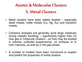
Atomic & Molecular Clusters 5. Metal Clusters

1. Atomic & Molecular Clusters5. Metal Clusters • Metal clusters have been widely studied – especially alkali metals, noble metals (Cu, Ag, Au) and transition metals. • Cohesive energies are generally quite large (relatively strong metallic bonding) – significantly higher than for rare gas or molecular clusters – so they may be studied in solution (colloidal suspensions), on surfaces or in inert matrices, as well as in the gas phase. • A number of models have been introduced to explain and predict the properties of metal clusters.

2. Energy IP W EA 1/R The Liquid Drop Model • A classical electrostatic model. • Cluster is approximated by a uniform conducting sphere. • Atomic positions and internal electronic structure ignored. • Predictions: As 1/R  0 (N ) {IP,EA}  W

3. {IP(R)W} / eV {WEA(R)} / eV 1/R / Å M. M. Kappes Chem. Rev. 1988, 88, 369.

4. Failures of the Liquid Drop Model • Deviations from 1/R dependence of IPs and EAs for small clusters. • IPs of Hg clusters show a discontinuity due to a size-dependent non-metal  metal transition (see later). • Some transition metals (where ionization involves removal of tightly bound d electrons, e.g. Fe, Ni) show small variation of IP/EA with size. • Magnetic effects (spin-spin interactions) also important for transition metals. • LDM does not reproduce fine structure in IP/EA variation with N (e.g. “even-odd alternation”) or explain the Magic Numbers in the mass spectra. • Require a Quantum Mechanical model with discrete electronic states  JELLIUM MODEL.

5. Mass Spectra and Magic Numbers • Mass spectra obtained by Knight and co-workers (1983-85), for alkali metal clusters, showed a number of peaks with high relative intensities  Magic Numbers. • Magic numbers (and origins) different from rare gas clusters.

6. The Jellium Model • Derived from nuclear structure theory. • Cluster approximated by a sphere with a uniform positively charged background, filled with an “electron gas” (valence electrons). • Valence electrons are delocalized – move in a smooth, attractive, central, mean field potential of spherical symmetry.

7. Positions of ionic cores are ignored. • This is justified if: • electrons are strongly delocalized • ionic background easily deformed • molten clusters? • Works best for monovalent simple metals • e.g. alkali metals, noble metals (Cu, Ag, Au). • Unlike the LDM, the jellium model is a quantum mechanical model • quantization of electron energy levels due to boundary conditions imposed by the potential. • Gives rise to electronic shell structure for metal clusters with up to several 1000s of atoms.

8. Empirical Jellium Models • Based on effective single-particle potentials (Knight, Clemenger). • Solve 1-electron Schrödinger Equation for an electron in a sphere, under the influence of an attractive central potential. • Wavefunction () is separable into radial and angular parts: n,,m(r,,)=Rn,(r).Y,m(,)

9. Solutions • Wavefunction and energies depend on quantum numbers: n = 1, 2, 3, …  = 0, 1, 2, … (no restriction on ) m =  … 0 … + (2 + 1)-degenerate • Note: the principal quantum number n is different from that used for atomic orbitals (follows convention of nuclear physics): nclust = natom -  • Jellium electronic levels (sets of degenerate orbitals) are labelled, by analogy with atomic orbitals: 1s, 1p, …, 2s, 2p … • Exact ordering of orbitals depends on the radial form of the potential.

10. U0 = EF + W R0 = Ratom.N1/3 The Woods-Saxon Potential • Obtained by fitting to high-level electronic structure calculations. • W-S potential is a finite well with rounded sides (intermediate between 3-D harmonic oscillator and 3-D square well).

11. 58 40 34 20 18 8 2 • Ordering of Levels: 1s < 1p < 1d < 2s < 1f < 2p < 1g … • Level Closings (no. of electrons) 2 8 18 20 34 4058 …

12. h + e MN MN+ Interpreting Mass Spectra of Metal Clusters • Low Energy Ionization • Magic numbers (intense peaks in MS) due to stable electron counts (filled jellium levels) of neutral clusters (MN). • N* = 8, 20, 40, 58 …

13. highly electronically excited + e MN+ high E h e evaporation of M atoms MN + (N-X)M MX+ • High Energy Ionization • Magic numbers due to stability of cationic clusters (MX+): N* = 9, 21, 41, 59 … • Note: Na8, Na9+ both have 8 electrons.

14. Breakdown of the Spherical Jellium Model • Fine structure is observed in the MS, IPs, EAs, polarizabilities etc., for even-electron counts other than those predicted by the (spherical) jellium model. • This is evidence for non-degenerate electronic sub-levels, which cannot be explained by the spherical jellium model. • Need to extend the model.

15. Iz = moment of inertia about z-axis etc. The Ellipsoidal Shell Model • Modification to spherical jellium model, introduced by Clemenger (1985). • Potential = a perturbed 3-D harmonic oscillator – analogous to Nilsson’s model (1955) for nuclear structure. • Ellipsoidal (“spheroidal”) distortion of cluster.

16. 1 =1 1 (np)4 (np)2 • Lowering of symmetry  loss of (2+1)-fold degeneracy of each jellium level (n). • m degeneracy is maintained in ellipsoidal (spheroidal) symmetry. • Oblate Spheroid E as |m| > ½-filled shell • Prolate Spheroid  E as |m| < ½-filled shell

17. Variation of Na Cluster Shape with Size

18. Comparison of structures of Na and Ar clusters

19. N1/3 Beyond the Jellium Model • Martin and co-workers (1991)* measured MS of NaN clusters (N 25,000). • Observed two series of periodic intensity variations: period  N1/3. * T. P. Martin et al., J. Phys. Chem.1991, 95, 6421.

20. Electronic Shells (N < 2000) • Electronic shells form due to bunching together of jellium levels. • Electronic shells = sets of nearly degenerate jellium levels.

21. jellium levels electronic shells band structure N • For larger metal clusters, electronic effects are relatively unimportant because electronic shells merge to form quasi-continuous bands (bulk-like band structure).

22. Geometric Shells (N > 2000) • Geometric shells correspond to complete concentric polyhedral shells of atoms – as for rare gas clusters. • Stability due to minimization of surface energy. • Alkali Metal Clusters – magic numbers are consistent with filling K geometric shells:

23. Examples of Geometric Shells rhombic dodecahedron (bcc) icosahedron truncated octahedron (fcc)

24. CaN+ N • Similar magic numbers have been observed for Ca clusters with up to 5000 atoms.* • MS magic numbers and fine structure (due to partial geometric shell formation) indicate that alkali metal clusters (with N > 2000) and Ca clusters have icosahedral shell structure. * T. P. Martin Physics Reports1996, 273, 199.

25. Al and In clusters form octahedral shell structures (fragments of fcc packing). • Geometric shell structure has also been found for many transition metal clusters (e.g. Co, Ni). • Electronic shell effects are relatively unimportant for TMs with unfilled d-orbitals as the onset of band structure occurs for quite low N. InN+

26. Microscopy Studies of Metal Clusters • A number of microscopy techniques can be applied to study metal clusters: • Electron Microscopy (TEM, SEM) • Scanning Tunnelling Microscopy (STM) • Atomic Force Microscopy (AFM) • Clusters must be immobilized on a substrate (e.g. graphite, amorphous-C, MgO, SiO2 – depending on the type of measurement). • Clusters are often passivated by surfactant (ligand) molecules. • Cluster-surface and cluster-ligand interaction may affect cluster structure (for small clusters).

27. 15 nm 4 nm Single Ag decahedron Multiply-twinned Ag fcc particle 3 nm 7 nm Intergrowth of 2 Au icosahedra Truncated octahedral Au fcc particle Marks decahedral Au particle Electron Micrographs of Ag and Au Particles

28. Mackay Icosahedra Quasi-spherical shape. Close-packed surface but strong internal strain. Maximizes the number of NN bonds favourable at small sizes Marks Decahedra Intermediate behaviour. Favourable at Intermediate sizes Fcc Polyhedra Non-spherical shape but no internal strain. Fewer NN bonds. Favourable at large sizes Energetics of pure Ag clusters

29. Insulator-Metal Transition in Hg Clusters • Rademann and Hensel (1987) measured IPs of Hg clusters as a function of size, N. • Explained in terms of a gradual transition: Insulating Semi-Conducting  Metallic in the region N ~ 13-70. • Consistent with spectroscopy and theoretical calculations.

30. Theory of Bonding in Hg Clusters • The free Hg atom has a closed shell: (6s)2(6p)0 • Small clusters are insulating “van der Waals clusters” – held together by dispersion forces. • As the cluster gets larger, the 6s and 6p levels broaden into bands (with widths Ws and Wp) • W as N • Insulator  Metal Transition occurs when the 6s and 6p bands overlap. • Before band overlap (intermediate N), the band gap (sp) may be comparable to the thermal energy (kT) • semi-conductor clusters • s-p hybridization occurs  covalent bonding

31. Size-dependent Electronic Structures of Hg Clusters