Download
1 / 18
180 likes | 347 Vues
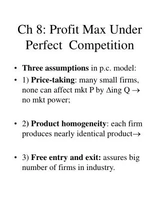
Ch 8: Profit Max Under Perfect Competition. Three assumptions in p.c. model: 1) Price-taking : many small firms, none can affect mkt P by ing Q no mkt power; 2 ) Product homogeneity : each firm produces nearly identical product

E N D
Ch 8: Profit Max Under Perfect Competition • Three assumptions in p.c. model: • 1) Price-taking: many small firms, none can affect mkt P by ing Q no mkt power; • 2) Product homogeneity: each firm produces nearly identical product • 3) Free entry and exit: assures big number of firms in industry.
More on Perfect Competition • Real-life examples: • Agricultural products • Oil. • P.C. is an ideal; useful starting point. • Also assume:
Profit Maximization • Profit-max extends beyond just p.c. mkt structure. • Define profit = TR – TC • (q) = R(q) – C(q), or • = R – C. • So firm picks q* where difference between TR and TC is greatest. • With graphs of TR and TC:
Three Curves in Figure 8.1 • TR: slope is MR • TC: slope is MC. • function: see inverse U-shape: • Max where: • 1) • 2) • 3) Rule: • pick -max q* where MR = MC.
Review Implications of Perfect Competition • First: keep terms straight: • Q = • D = • q = • d = • Market D is downward sloping but demand curve faced by individual firm is perfectly elastic (horizontal). • So: firm demand curve is same is its MR curve.
Further Implications • Recall: firm’s demand curve is its MR curve. • This means that P = MR. • So profit-max rule: pick -max q* where MC = MR = P. • Also, since P = MR for each q, then P = MR = AR.
FURTHER Details • Revise rule: pick -max q* where MR = MC AND MC is rising. • Note: • Short Run profit for p.c. firm: • P - ATC at q* = avg profit per unit of q. • Explain: • Total at q* = q* avg. .
Firm’s SR Shutdown Decision • Situation: What if the SR -max q* results in losses? • Firm must choose (1) vs (2): • 1) Continue producing at q*: • 2) Shutdown in SR:
SR Shutdown Rule • Firm must know: at q*, what is: • P, • ATC, and • AVC. • Rule: If 0 in SR: • continuing producing q* as long as P AVC. • In LR:
Competitive Firm’s SR Supply Curve • Supply Curve: shows q produced at each possible price. • SR supply curve: the firm’s MC curve for all points where MC AVC • I.e., -max q* is where P AVC. • Remember “trigger” for shutdown in SR implies that MC curve has an irrelevant part (where MC P).
Firm’s Response to Price of Input • Consider: price input causes MC at each q shift up to left of MC curve. • See Figure 8.7: • Start at P = $5 with MC1; so q* = q1. • Now: price input causes MC: • Shifts MC up to left. • Causes q*.
SR Market Supply Curve • Shows: amount of Q the industry will produce in SR at each possible price. • Sum SR supply curves for firms using horizontal summation. • That is: at each possible price, sum up total quantity supplied by each firm. • See Figure 8.9. • (Note: for each firm: as q es, individual MC curves no .).
Price Elasticity of Market Supply • ES = %Qs/1%P = • (Q/Q) / (P/P). • ES 0 always because SMC slopes upward. • If MC a lot in response to Q, then ES is low. • Extreme cases: • Perfectly inelastic S: • Perfect elastic S:
Producer Surplus in SR • Concept analogous to CS. • For rising MC: P MC for every unit of q except last one produced. • For a firm (see Figure 8.11): • For all units produced (up to q*): • Measures area above MC schedule (S curve) and below mkt price.
LR Competitive Equilibrium • If each firm earns zero economic , each firm is in LR equilibrium. • Three conditions: • 1. All firms in industry are profit-maximizing. • 2. No firm has incentive to enter or leave industry (due to = 0). • 3. P is that which equates QS = QD in market.
Adjustment from SR to LR Equilibrium • Firm starts in SR equilibrium. • Positive profits induce new firms to entire industry. • This causes market P to fall. • This causes firm’s MR line to fall, until profits = 0 again. • Key: firms enter as long as P AVC • Note: in this case, MC no shift due to constant cost assumption. • LR choice of q*: • where LMC = P = MR = LAC. • Key is LMC=LAC.
Economic Rent • Economic Rent: • For an industry: economic rent same as LR producer surplus. • For a fairly fixed factor (like land): • In LR in a competitive mkt:
Industry’s LR Supply Curve • Cannot just sum horizontally because as price es, # firms in industry es. Must connect the zero-profit points. • Shape of LR supply curve: depends on whether (and in what direction) the es in each firm’s q causes es in input prices. • Constant cost industry: As q and Q , input prices no so firm’s MC, AVC, and ATC NO shift as q changes. • SO: LR industry supply curve is flat (perfectly horizontal).