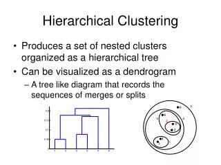
Hierarchical Clustering
Hierarchical Clustering. Leopoldo Infante Pontificia Universidad Católica de Chile. Reunión Latinoamericana de Astronomía Córdoba, septiembre 2001. Introduction The Two-point Correlation Function Clustering of Galaxies at Low Redshifts - SDSS results-

Hierarchical Clustering
E N D
Presentation Transcript
Hierarchical Clustering Leopoldo Infante Pontificia Universidad Católica de Chile Reunión Latinoamericana de Astronomía Córdoba, septiembre 2001
Introduction The Two-point Correlation Function Clustering of Galaxies at Low Redshifts -SDSS results- Evolution of Clustering -CNOC2 results- Clustering of Small Groups of Galaxies The ro - d diagram
Rich Clusters Bias Groups Bias Galaxies Bias
How do we characterizeclustering? Correlation Functions and/or Power Spectrum
Random Distribution 1-Point 2-Point N-Point dV1 Clustered Distribution r 2-Point dV2
Continuous Distribution Fourier Transform Since P depends only on k
In Practice 2-Dimensions - Angles Estimators B A
Assumed Power Law 3-D Correlation Function Proper Correlation distance Clustering evolution index Proper Correlation length Assumed Power Law Angular Correlation Function
Inter-system Separation, d Space density of galaxy systems Mean separation of objects As richer systems are rarer, d scales with richness or mass of the system
CLUSTERINGMeasurements from Galaxy CatalogsandPredictions from Simulations
Sloan Digital Sky Survey • 2.5m Telescope • Two Surveys • Photometric • Spectroscopic • Expect • 1 million galaxies with spectra • 108 galaxies with 5 colors • Current results • Two nights • Equatorial strip, 225 deg.2 • 2.5 million galaxies
Angular Clustering • Correlations on a given angular scale probe physical scales of all sizes. • Fainter galaxies are on average further away, so probe larger physical scales
Power law over 2 orders of magnitude • Correlation in faintest bin correspond to larger physical scales • less clustered
CNOC2 Survey Measures clustering evolution up to z 0.6 for Late and Early type galaxies. 1.55 deg.2 ~ 3000 galaxies 0.1 < z < 0.6 Redshifts for objects with Rc< 21.5 Rc band, MR < -20 rp<10h-1Mpc SEDs are determined from UBVRcIc photometry
Projected Correlation Length
Clustering of Galaxy Clusters Richer clusters are more strongly clustered. Bahcall & Cen, 92, Bahcall & West, 92 ro=0.4 dc=0.4 nc-1/3 However this has been disputed Incompleteness in cluster samples (Abell, etc.) APM cluster sample show weaker trend
N body simulations • Bahcall & Cen, ‘92, ro dc • Croft & Efstathiou, ‘94, ro dc but weaker • Colberg et al., ‘00, (The Virgo Consortium) • 109 particles • Cubes of 2h-1Gpc (CDM) 3h-1Gpc (CDM) CDM =1.0 =0.0 h=0.5 =0.21 8=0.6 CDM =0.3 =0.7 h=0.5 =0.17 8=0.9
CDM dc = 40, 70, 100, 130 h-1Mpc Dark matter
Clustering and Evolution of Small Groups of Galaxies
Objective: Understand formation and evolution of structures in the universe, from individual galaxies, to galaxies in groups to clusters of galaxies. • Main data: SDSS, equatorial strip, RCS, etc. • Secondary data: Spectroscopy to get redshifts. • Expected results: dN/dz as a function of z, occupation numbers (HOD) and mass. • Derive ro and d=n-1/3 Clustering Properties
Bias • The galaxy distribution is a bias tracer of the matter distribution. • Galaxy formation only in the highest peaks of density fluctuations. • However, matter clusters continuously. • In order to test structure formation models we must understand this bias.
Halo Occupation Distribution, HOD Bias, the relation between matter and galaxy distribution, for a specific type of galaxy, is defined by: • The probability, P(N/M), that a halo of virial mass M contains N galaxies. • The relation between the halo and galaxy spatial distribution. • The relation between the dark matter and galaxy velocity distribution. This provides a knowledge of the relation between galaxies and the overall distribution of matter, the Halo Occupation Distribution.
In practice, how do we measure HOD? • Detect pairs, triplets, quadruplets etc. n2 in SDSS catalog. • Measure redshifts of a selected sample. • With z and N we obtain dN/dz We are carrying out a project to find galaxies in small groups using SDSS data.
Collaborators: M. Strauss N. Bahcall J. Knapp M. Vogeley R. Kim R. Lupton & Sloan consortium
Note strips • The Data • Equatorial strip, 2.5100 deg2 • Seeing 1.2” to 2” • Area = 278.13 deg2 • Mags. 18 < r* < 20 • Ngalaxies = 330,041
De-reddened Galaxy Counts Thin lines are counts on each of the 12 scanlines dlogN/dm=0.46 Turnover at r* 20.8
Selection of Galaxy Systems • Find all galaxies within angular separation 2”<<15” (~37h-1kpc) • and 18 < r* < 20 • Merge all groups which have members in common. • Define a radius group: RG • Define distance from the group o the next galaxy; RN • Isolation criterion: RG/RN 3 Sample 1175 groups with more than 3 members 15,492 pairs Mean redshift = 0.22 0.1
Galaxy pairs, examples Image imspection shows that less than 3% are spurious detections
Main Results arcsec arcsec A = 13.54 0.07 = 1.76 A = 4.94 0.02 = 1.77
Secondary Results galaxies pairs triplets • Triplets are more clustered than pairs • Hint of an excess at small angular scales
Space Clustering Properties-Limber’s Inversion- Calculate correlation amplitudes from () Measure redshift distributions, dN/dz De-project () to obtain ro, correlation lengths Compare ro systems with different HODs SDSS CNOC2
The ro - d relation Amplitude of the correlation function Correlation scale Mean separation As richer systems are rarer, d scales with richness or mass of the system
Rich Abell Clusters: • Bahcall & Soneira 1983 • Peacock & West 1992 • Postman et al. 1992 • Lee &Park 2000 • APM Clusters: • Croft et al. 1997 • Lee & Park 2000 EDCC Clusters: Nichol et al. 1992 • X-ray Clusters: • Bohringer et al. 2001 • Abadi et al. 1998 • Lee & Park 2000 LCDM (m=0.3, L=0.7, h=0.7) SCDM (m = 1, L=0, h=0.5) Governato et al. 2000 Colberg et al. 2000 Bahcall et al. 2001 • Groups of Galaxies: • Merchan et al. 2000 • Girardi et al. 2000
CONCLUSIONS We use a sample of 330,041 galaxies within 278 deg2, with magnitudes 18 < r* < 20, from SDSS commissioning imaging data. We select isolated small groups. We determine the angular correlation function. We find the following: • Pairs and triplets are ~ 3 times more strongly clustered than galaxies. • Logarithmic slopes are = 1.77 ± 0.04 (galaxies and pairs) • () is measured up to 1 deg. scales, ~ 9 h-1Mpc at <z>=0.22. No breaks. • We find ro= 4.2 ± 0.4 h-1Mpc for galaxies and 7.8 ± 0.7 h-1Mpc for pairs • We find d = 3.7 and 10.2 h-1Mpc for galaxies and pairs respectively. • LCDM provides a considerable better match to the data Follow-up studies dN/dz and photometric redshifts. Select groups over > 1000 deg2 area from SDSS