Spin-spin coupling analysis The last parameter that we will discuss concerning the

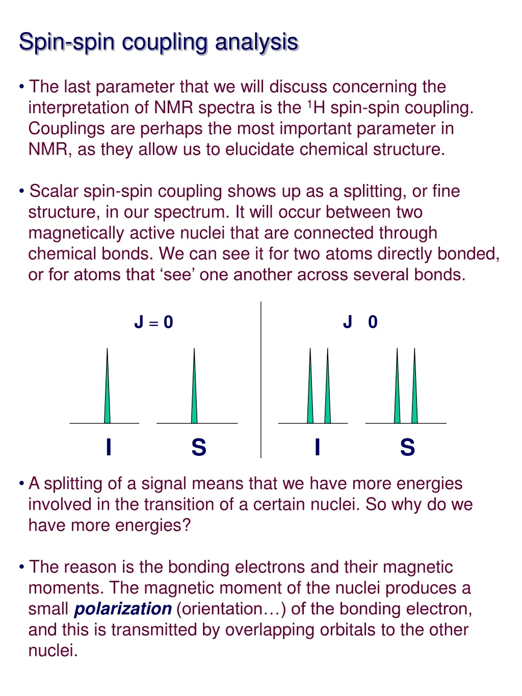
1. Spin-spin coupling analysis • The last parameter that we will discuss concerning the • interpretation of NMR spectra is the 1H spin-spin coupling. • Couplings are perhaps the most important parameter in • NMR, as they allow us to elucidate chemical structure. • Scalar spin-spin coupling shows up as a splitting, or fine • structure, in our spectrum. It will occur between two • magnetically active nuclei that are connected through • chemical bonds. We can see it for two atoms directly bonded, • or for atoms that ‘see’ one another across several bonds. • A splitting of a signal means that we have more energies • involved in the transition of a certain nuclei. So why do we • have more energies? • The reason is the bonding electrons and their magnetic • moments. The magnetic moment of the nuclei produces a • small polarization (orientation…) of the bonding electron, • and this is transmitted by overlapping orbitals to the other • nuclei. J  0 J = 0 I S I S

2. Spin-spin coupling (continued) • We can explain this better by looking at HF: • The nuclear magnetic moment of 19F polarizes the F bonding • electron (up), which, since we are following quantum • mechanics rules, makes the other electron point down (the • electron spins have to be antiparallel). • Now, the since we have different states for the 1H electrons • depending on the state of the 19F nucleus, we will have • slightly different energies for the 1H nuclear magnetic • moment (remember that the 1s electron of the 1H generates • an induced field…). • This difference in energies for the 1H result in a splitting of • the 1H resonance line. 19F 1H Nucleus Bo Electron 19F 1H

3. Spin-spin coupling (…) • We can do a similar analysis for a CH2 group: • The only difference here is that the C bonds are hybrid bonds • (sp3), and therefore the Pauli principle and Hundi’s rules • predict that the two electrons will be parallel. • Irrespective of this, the state of one of the 1H nuclei is • transmitted along the bonds to the other 1H, and we get a • splitting (a doublet in this case…). The energy of the • interactions between two spins A and B can be found by the • relationship: 1H 1H Bo C E = JAB * IA * IB

4. Spin-spin coupling (…) • IAandIBare the nuclear spin vectors, and are proportional to • mAandmB, the magnetic moments of the two nuclei.JABis • the scalar coupling constant. So we see a very important • feature of couplings. It does not matter if we have a 60, a • 400, or an 800 MHz magnet,the coupling constants are • always the same!!! • Lets do a more detailed analysis in term of the energies. Lets • think a two energy level system, and the transitions for nuclei • A. When we have no coupling (J = 0), the energy involved in • either transition (A1 or A2) is equal (no spin-spin interaction). • The relative orientations of the nuclear moments does not • matter. We see a single line (two with equal frequency). • When J > 0, the energy levels of the spin system will be • either stabilized or destabilized.Depending on the relative • orientations of the nuclear moments, the energies for the A1 • and A2 transition will change giving two different frequencies • (two peaks for A). A X J > 0 A X J = 0 E4 E3 E2 E1 A2 A2 Bo E A1 A1

5. Spin-spin coupling (…) • We choose J > 0 as that related to antiparallel nuclear • moments (lower energy). The energy diagram for J < 0 would • then be: • If we look at it as a stick spectrum for either case we get: • As mentioned before, the choice of positive or negative J is a • definition. However, we see that we won’t be able to tell if we • have a positive or negative J, because the lines in the • spectrum corresponding to the different transitions basically • change places. Unless we are interested in studying the • energies, this is not important for structure elucidation… A X J = 0 A X J < 0 E4 E3 E2 E1 A2 A2 Bo E A1 A1 J > 0 J < 0 J = 0 A2 A1 A2 A2 A1 A1 n A1n A2 n A1 = n A2 n A2n A1

6. Spin-spin coupling (…) • We can do a quantitative analysis of the energy values from • to gain some more insight on the phenomenon. The base • energies of the system are related to the Larmor • frequencies, and the spin-spin interaction is JAX: • So if we now consider the transitions that we see in the • spectrum, we get: • This explains the lines in our spectrum quantitatively… J > 0 E4 = 1/2nA + 1/2nB + 1/4 JAX E3 = 1/2nA - 1/2nB - 1/4 JAX E2 = - 1/2nA + 1/2nB - 1/4 JAX E1 = - 1/2nA - 1/2nB + 1/4 JAX 4 I2 A1 2 3 A2 I1 1 A1 = E4 - E2 = nA - 1/2 JAX A2 = E3 - E1 = nA + 1/2 JAX I1 = E2 - E1 = nB - 1/2 JAX I2 = E4 - E3 = nB + 1/2 JAX

7. Analysis of 1st order systems • Now we will focus on the simplest type of coupling we can • have, which is one of the limits of a more complex quantum • mechanical description. • Lets say that we have ethylacetate. In this molecule, the • resonance of the CH3 from the ethyl will be ~ 1.5, while that • for the CH2 will be ~ 4.5 ppm. In most spectrometers this • means that the difference in chemicals shifts, Dn, will be a lot • bigger than the coupling constant J, which for this system is • ~ 7 Hz. In this case, we say that we have a first order spin • system. • If we analyze the system in the same way we did the simple • AX system, we will see that each 1H on the CH2 will see 4 • possible states of the CH31Hs, while each 1H on the CH3 • will see 3 possible states of the CH2 protons. We have to • keep in mind that the two 1Hs of the CH2 and the three 1Hs of • the CH3 are equivalent. • In order to see this better, we can build a diagram that has • the possible states of each 1H type in EtOAC: aaa aab aba baa abb bab bba bbb aa ab ba bb CH3 CH2

8. 1st order systems (continued) • If we generalize, we see that if a certain nuclei A is coupled • to n identical nuclei X (of spin 1/2), A will show up as n + 1 • lines in the spectrum. Therefore, the CH2 in EtOAc will show • up as four lines, or a quartet. Analogously, the CH3 in EtOAc • will show up as three lines, or a triplet. • The separation of the lines will be equal to the coupling • constant between the two types of nuclei (CH2’s and CH3’s in • EtOAc, approximately 7 Hz). • If we consider the diagram of the possible states of each • nuclei, we can also see what will be the intensities of the • lines: • Since we have the same probability of finding the system in • any of the states, and states in the same rows have equal • energy, the intensity will have • a ratio 1:2:1 for the CH3, and • a ratio of 1:3:3:1 for the CH2: CH3 CH2 J (Hz) CH3 CH2 4.5 ppm 1.5 ppm

9. 1st order systems (…) • These rules are actually a generalization of a more general • rule. The splitting of the resonance of a nuclei A by a nuclei • X with spin number I will be 2I + 1. • Therefore, if we consider -CH2-CH3, • and the effect of each of the CH3’s • 1Hs, and an initial intensity of 8, • we have: • Since the coupling to each 1H of the CH3 is the same, the • lines will fall on top of one another. • In general, the number of lines in these cases will be a • binomial expansion, known as the Pascal Triangle: 8 Coupling to the first 1H (2 * 1/2 + 1 = 2) 4 4 Coupling to the second 1H 2 22 2 Coupling to the third 1H 1 111 111 1 1 : n / 1 : n ( n - 1 ) / 2 : n ( n - 1 ) ( n - 2 ) / 6 : ...

10. 1st order systems (…) • Here n is the number of equivalent • spins 1/2 we are coupled to: The • results for several n’s: • In a spin system in which we have a certain nuclei coupled to • more than one nuclei, all first order, the splitting will be • basically an extension of what we saw before. • Say that we have a CH (A) coupled to a CH3 (M) with a JAM • of 7 Hz, and to a CH2 (X) with a JAX of 5 Hz. We basically • go in steps. First the big coupling, which will give a quartet: • Then the small coupling, • which will split each line • in the quartet into a triplet: • This is called a triplet of quartets (big effect is the last…). 1 1 1 1 2 1 1 3 3 1 1 4 6 4 1 7 Hz 5 Hz

11. 1st order systems (…) • Lets finish our analysis of 1st order system with some pretty • simple rules that we can use when we are actually looking at • 1D 1H spectra. • To do that, say that again • we have a system in with a • CH (A) coupled to two CH’s • (M and R) with a JAM of 8 Hz • and JAR of 5 Hz, and to a • CH2 (X) with a JAX or 6 Hz: • The first rule is that if we have a clear-cut first order system, • the chemical shift of nuclei A, dA, is always at the center of • mass of the multiplet. • The second one is that no matter how complicated the • pattern may end up being, the outermost splitting is always • the smallest coupling for nuclei A. We can measure it without • worrying about picking the wrong peaks from the pattern. 8 Hz 5 Hz 6 Hz dA 5 Hz

12. The Karplus equation • The most common coupling constant we’ll see is the three- • bond coupling, or 3J: • As with the 1J or 2J, the coupling arises from the interactions • between nuclei and electron spins. 1J and 3J will hold the • same sign, while 2J will have opposite sign. • However, the overlap of electron and nuclear wavefunctions • in the case of 3J couplings will depend on the dihedral angle • <f> formed between the CH vectors in the system. • The magnitude of the 3J couplings will have a periodic • variation with the torsion anlge, something that was first • observed by Martin Karplus in the 1950’s. 1H C f C 1H

13. The Karplus equation (...) • The relationship can be expressed as a cosine series: • Here A, B, and C are constants that depend on the topology • of the bond (i.e., on the electronegativity of the substituents). • Graphically, the Karplus equation looks like this: • A nice ‘feature’ of the Karplus equation is that we can • estimate dihedral angles from 3J coupling constants. Thus, a • variety of A, B, and C parameters have been determined for • peptides, sugars, etc., etc. 3JHH = A · cos2( f) + B · cos( f ) + C f 3JHH (Hz) f (o)

14. The Karplus equation (...) • As an example, consider an SN2 inversion reaction we do in • our lab. We go from a trans to a cisb-lactam. • The <fHH> in the trans is 137.3o, while in the cis • product it is 1.9o. So, we know we have inversion... 3JHH = 1.7 Hz N3- 3JHH = 5.4 Hz

15. 2nd order systems - The AB system • What we have been describing so far is a spin system in • which Dn >> J, and as we said, we are analyzing one of the • limiting cases that QM predict. • As Dn approaches J, there will be more transitions of similar • energy and thus our spectrum will start showing more • signals than our simple analysis predicted. Furthermore, the • intensities and positions of the lines of the multiplets will be • different from what we saw so far. • Lets say that we have two • coupled nuclei, A and B, • and we start decreasing • our Bo. Dn will get smaller • with J staying the same. • After a while, Dn ~ J. What • we see is the following: • What we did here is to • start with an AX system • (the chemical shifts of • A and X are very different) • and finish with an AB • system, in which Dn ~ J. • Our system is now a second • order system. We have effects that are not predicted by the • simple multiplicity rules that we described earlier. Dn >> J Dn = 0

16. The AB system (continued) • Thus, the analysis of an AB system is not as straightforward • as the analysis of an AX system. A full analysis cannot be • done without math and QM, but we can describe the results. • A very simple way to determine • if we have an AB system is by • looking at the roofing effect: • coupled pairs will lean towards • each other, making a little roof: • As with an AX system, JAB • is the separation between • lines 1 and 2 or 3 and 4: • Now, the chemical shifts of nuclei A and B are not at the • center of the doublets. They will be at the center of mass of • both lines. Being Dnthe nA - nB chemical shift difference, nA • and nB will be: nA nZ nB A B 1 2 3 4 | JAB | = | f1 - f2 | = | f3 - f4 | • Peak intensities can be • computed similarly: Dn2 = | ( f1 - f4 ) ( f2 - f3 ) | nA= nZ - Dn / 2 nB= nZ + Dn / 2 I2 I3 | f1 - f4 | = = I1 I4 | f2 - f3 |

17. Magnetic and chemical equivalence • Before we get deeper into analysis of coupling patterns, lets • pay some more attention to naming conventions, as well as • to some concepts regarding chemical and magnetic • equivalence. • Our first definition will be that of a spin system. We have a • spin system when we have a group of n nuclei (with I = 1/2) • that is characterized by no more than n frequencies • (chemical shifts) ni and n ( n - 1 ) / 2 couplings Jij. The • couplings have to be within nuclei in the spin system. • We start by defining magnetic equivalence by analyzing • some examples. Say that we have an ethoxy group (-O-CH2- • CH3). • As we saw last time, we can do a very simple first order • analysis of this spin system, because we assumed that all • CH2 protons were ‘equal,’ and all CH3 protons were ‘equal.’ Is • this true? • We can easily see that they are chemically equivalent. • Additionally, we have free rotation around the bond, which • makes their chemical shifts and couplings equal.

18. Magnetic equivalence (continued) • Since the 1Hs can change places, they will alternate their • chemical shifts (those bonded to the same carbon), and we • will see an average. • The same happens for the J couplings. We’ll see an average • of all the JHH couplings, so in effect, the coupling of any • proton in CH2 to any proton in the CH3 will be the same. • If we introduce some notation, and remembering that d(CH2) • is >> d(CH3), this would be an A2X3 system: We have 2 • magnetically equivalent 1Hs on the CH2, and 3 on the CH3. • The 2JHH coupling (that is, the coupling between two nuclei • bound to the same carbon) is zero in this case, because the • energies for any of the three (or two) protons is the same. • Finally, we use A to refer to the CH2 protons, and X to refer • to the CH3 protons because they have very different ds. We • usually start with the letter A for the most deshielded spin. • Difluoromethane is another example of an ‘AX’ type system: • In this case, 1Hs and 19Fs are equal not due to rotation, but to • symmetry around the carbon. It’s an A2X2 system.

19. Magnetic equivalence (…) • For CH2F2, we can also compare the couplings to check that • the 1Hs and 19Fs are equivalent: JH1F1 = JH1F2 = JH2F1 = JH2F2. • All due to their symmetry... • Now, what about the • the 1Hs and 19Fs in • 1,1-difluoroethene? • Here we also have symmetry, but no rotation. The two 1Hs • and the two 19Fs are chemically equivalent, and we can • easily see that dHa = dHb and dFa = dFb. • However, due to the geometry of this compound, JHaFa • JHaFb. Analogously, JHbFa JHbFb. • Furthermore, since the couplings are different, the energy • levels for Ha and Hb are different (not degenerate anymore • as in CH3), and we have JHaHb 0. • If we consider all the possible couplings we have, we have • three different couplings for each proton. For Ha, we have • JHaFa, JHaFb, and JHaHb. For Hb, we have JHbFa, JHbFb, and • JHbHa. This means more than the eight possible transitions • (2*2*2) in the energy diagram, and an equal number of • possible lines in the spectrum!

20. Magnetic equivalence (…) • These are representative spectra (only the 1H spectrum is • shown) of CH2F2 and F2C=CH2: • A system like this is not an A2X2, but an AA’XX’ system. We • have two A nuclei with the same chemical shift but that are • not magnetically equivalent. The same goes for the X nuclei. • The following are other examples of AA’XX’ systems: CH2F2 H2C=CF2

21. Energy diagrams for 2nd order systems • From what we’ve seen, most cases of magnetic non- • equivalence give rise to 2nd order systems, because we will • have two nuclei with the same chemical environment and the • same chemical shift, but with different couplings (AA’ type…). • We have analyzed qualitatively how a 2nd order AB looks like. • In an AB system we have two spins in which Dd ~ JAB. The • energy diagram looks a lot like a 1st order AX system, but the • energies involved (frequencies) • and the transition probabilities • (intensities) are such that we • get a messier spectrum: • Some examples of AB systems: bb B A ab ba A B aa

22. Transition from 1st order to 2nd order • The following is a neat experimental example of how we go • from a 1st order system to a 2nd order system. The protons • in the two compounds have the same ‘arrangement’, but as • Dd approaches JAB, we go from, in this case, A2X to A2B: • Most examples have ‘ringing’ and are obtained at relatively • low fields (60 MHz) because at these fields 2nd order effects • are more common…

23. 2nd order systems with more than 2 spins. • Now, lets analyze 2nd order systems with more than 2 spins. • We already saw an example, the A2X system and the A2B • system. The A2X system is 1st order, and is therefore easy to • analyze. • The A2B is 2nd order, and energy levels includes transitions • for what are known as symmetric and antisymmetric • wavefunctions. They are related with the symmetry of the • quantum mechanical wavefunctions describing the system. • In any case, we have additional transitions from the ones we • see in a A2X system: • We now have 9 lines in the A2B system, instead of the 5 we • have in the A2X system (we have to remember that in the • A2X many of the transitions are of equivalent energy…). A2B A2X bbb bbb bba bab abb b(ab+ba) abb b(ab-ba) baa aba aab baa a(ab+ba) a(ab-ba) anti symmetric aaa aaa symmetric

24. More than 2 spins (continued) • An A2B (or AB2) spectrum • will look like this: • Another system that we will encounter is the ABX system, in • which two nuclei have comparable chemical shifts and a third • is far from them. The energy levels look like this: bb X(a) A B bb ba ab A B A B ba ab aa A B X(b) ab

25. More than 2 spins (…) • In a ABX spectrum, we will have 4 lines for the A part, 4 lines • for the B part, and 6 lines for the X part: • ABX spin systems are very common in trisubstituted • aromatic systems. • The last system we will discuss is the AA’BB’ system, that • we saw briefly at the beginning (actually, we saw AA’XX’…).

26. More than 2 spins (…) • In anAA’BB’/AA’XX’system we have 2 pairs of magnetically • non-equivalent protons with the same chemical shift. The • energy diagram for such as system is: • We see that we can have a total of 12 transitions for each • spin (the AA’ part or the BB’ part). However, some of the • energies are the same (they are degenerate), so the total • number of lines comes down to 10 for each, a total of 20! • In an AA’XX’ we see two sub-spectra, one for the AA’ part • and one for the XX’ part. In a AA’BB’ we see everything on • the same region of the spectrum. bbbb abbb babb bbab bbba aabb abab baab baba bbaa abba aaab aaba abaa baaa anti symmetric aaaa symmetric

27. More than 2 spins (…) • Some examples of spin systems giving rise to AA’XX’ and • AA’BB’ patterns are given below. • A typical AA’BB’ spectrum is that of ODCB, orthodichloro • benzene. There are so many signals and they are so close to • each other, that this compound is used to calibrate instrument • resolution.

28. Common cases for 2nd order systems • So what type of systems we will commonly encounter that will • give rise to 2nd order patterns? Most of the times, aromatics • will give 2nd order systems because the chemical shift • differences of several of the aromatic protons will be very • close (0.1 to 0.5 ppm), and JHH in aromatics are relatively • large (9 Hz for 3J, 3 Hz for 4J, and 0.5 Hz for 5J). • For other compounds, the general rule is that if protons in • similar environments are ‘fixed’ (that is, they have restricted • rotation), we will most likely have 2nd order patterns. • A typical example of this, generally of an ABX system, are • pro-R and pro-S (i.e., diastereotopic) protons of methylenes • next to a chiral center: • In this case, we will have two protons that • are coupled to one another (because they • are different, A and B), they will have very • similar chemical shifts, and can be coupled • to other spins. For example, the oxetane • protons in taxol: