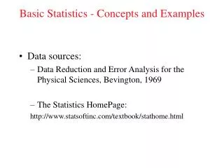
Basic Statistics - Concepts and Examples
Basic Statistics - Concepts and Examples. Data sources: Data Reduction and Error Analysis for the Physical Sciences, Bevington, 1969 The Statistics HomePage: http://www.statsoftinc.com/textbook/stathome.html. Elementary Concepts.

Basic Statistics - Concepts and Examples
E N D
Presentation Transcript
Basic Statistics - Concepts and Examples • Data sources: • Data Reduction and Error Analysis for the Physical Sciences, Bevington, 1969 • The Statistics HomePage: http://www.statsoftinc.com/textbook/stathome.html
Elementary Concepts • Variables: Variables are things that we measure, control, or manipulate in research. They differ in many respects, most notably in the role they are given in our research and in the type of measures that can be applied to them. • Observational vs. experimental research. Most empirical research belongs clearly to one of those two general categories. In observational research we do not (or at least try not to) influence any variables but only measure them and look for relations (correlations) between some set of variables. In experimental research, we manipulate some variables and then measure the effects of this manipulation on other variables. • Dependent vs. independent variables. Independent variables are those that are manipulated whereas dependent variables are only measured or registered.
Variable Types and Information Content Measurement scales. Variables differ in "how well" they can be measured. Measurement error involved in every measurement, which determines the "amount of information” obtained. Another factor is the variable’s "type of measurement scale." • Nominal variables allow for only qualitative classification. That is, they can be measured only in terms of whether the individual items belong to some distinctively different categories, but we cannot quantify or even rank order those categories. Typical examples of nominal variables are gender, race, color, city, etc. • Ordinal variables allow us to rank order the items we measure in terms of which has less and which has more of the quality represented by the variable, but still they do not allow us to say "how much more.” A typical example of an ordinal variable is the socioeconomic status of families. • Interval variables allow us not only to rank order the items that are measured, but also to quantify and compare the sizes of differences between them. For example, temperature, as measured in degrees Fahrenheit or Celsius, constitutes an interval scale. • Ratio variables are very similar to interval variables; in addition to all the properties of interval variables, they feature an identifiable absolute zero point, thus they allow for statements such as x is two times more than y. Typical examples of ratio scales are measures of time or space. Most statistical data analysis procedures do not distinguish between the interval and ratio properties of the measurement scales.
Systematic and Random Errors • Error: Defined as the difference between a calculated or observed value and the “true” value • Blunders: Usually apparent either as obviously incorrect data points or results that are not reasonably close to the expected value. Easy to detect. • Systematic Errors: Errors that occur reproducibly from faulty calibration of equipment or observer bias. Statistical analysis in generally not useful, but rather corrections must be made based on experimental conditions. • Random Errors: Errors that result from the fluctuations in observations. Requires that experiments be repeated a sufficient number of time to establish the precision of measurement.
Accuracy vs. Precision • Accuracy: A measure of how close an experimental result is to the true value. • Precision: A measure of how exactly the result is determined. It is also a measure of how reproducible the result is. • Absolute precision: indicates the uncertainty in the same units as the observation • Relative precision: indicates the uncertainty in terms of a fraction of the value of the result
Uncertainties • In most cases, cannot know what the “true” value is unless there is an independent determination (i.e. different measurement technique). • Only can consider estimates of the error. • Discrepancy is the difference between two or more observations. This gives rise to uncertainty. • Probable Error: Indicates the magnitude of the error we estimate to have made in the measurements. Means that if we make a measurement that we “probably” won’t be wrong by that amount.
Parent vs. Sample Populations • Parent population:Hypothetical probability distribution if we were to make an infinite number of measurements of some variable or set of variables. • Sample population:Actual set of experimental observations or measurements of some variable or set of variables. • In General: (Parent Parameter) = lim (Sample Parameter) When the number of observations, N, goes to infinity. N ->∞
some univariate statistical terms: mode: value that occurs most frequently in a distribution (usually the highest point of curve) may have more than one mode in a dataset median: value midway in the frequency distribution …half the area of curve is to right and other to left mean: arithmetic average …sum of all observations divided by # of observations poor measure of central tendency in skewed distributions range: measure of dispersion about mean (maximum minus minimum) when max and min are unusual values, range may be a misleading measure of dispersion
histogram is a useful graphic representation of information content of sample or parent population many statistical tests assume values are normally distributed not always the case! examine data prior to processing from: Jensen, 1996
Deviations The deviation, di, of any measurement xi from the mean m of the parent distribution is defined as the difference between xi and m Average deviation, a, is defined as the average of the magnitudes of the deviations, which is given by the absolute value of the deviations.
variance: average squared deviation of all possible observations from a sample mean (calculated from sum of squares) n s2i = lim [1/NS (xi - µ)2] N->∞ i=1 where: µ is the mean, xiis observed value, and N is the number of observations n S (xi - µ)2 s2i = Number decreased from N to N - 1for the “sample” variance as µ is used in the calculation i=1 N- 1 standard deviation: positive square root of the variance small std dev: observations are clustered tightly around a central value large std dev: observations are scattered widely about the mean
Sample Mean and Standard Deviation Sample Mean Our best estimate of the standard deviation s would be from: But we cannot know the true parent mean µ so the best estimate of the sample variance and standard deviation would be: Sample Variance
Distributions • Binomial Distribution:Allows us to define the probability, p, of observing x a specific combination of n items, which is derived from the fundamental formulas for the permutations and combinations. • Permutations: Enumerate the number of permutations, Pm(n,x), of coin flips, when we pick up the coins one at a time from a collection of n coins and put x of them into the “heads” box.
Distributions - con’t. • Combinations: Relates to the number of ways we can combine the various permutations enumerated above from our coin flip experiment. Thus the number of combinations is equal to the number of permutations divided by the degeneracy factor x! of the permutations.
Probability and the Binomial Distribution Coin Toss Experiment: If p is the probability of success (landing heads up) is not necessarily equal to the probability q = 1 - p for failure (landing tails up) because the coins may be lopsided! The probability for each of the combinations of x coins heads up and n -x coins tails up is equal to pxqn-x. The binomial distribution can be used to calculate the probability: The coefficients PB(x,n,p) are closely related to the binomial theorem for the expansion of a power of a sum:
Mean and Variance: Binomial Distribution The mean µ of the binomial distribution is evaluated by combining the definition of µ with the function that defines the probability, yielding: The average of the number of successes will approach a mean value µ given by the probability for success of each item p times the number of items. For the coin toss experiment p=1/2, half the coins should land heads up on average. If the the probability for a single success p is equal to the probability for failure p=q=1/2, the final distribution is symmetric about the mean and mode and median equal the mean. The variance, s2 = m/2.
Other Probability Distributions: Special Cases • Poisson Distribution:An approximation to the binomial distribution for the special case when the average number of successes is very much smaller than the possible number i.e. µ << n because p << 1. • Important for the study of such phenomena as radioactive decay. Distribution is NOT necessarily symmetric! Data are usually bounded on one side and not the other. Advantage is that s2 = m. µ = 1.67 s = 1.29 µ = 10.0 s = 3.16
Gaussian or Normal Error Distribution Details • Gaussian Distribution:Most important probability distribution in the statistical analysis of experimental data. functional form is relatively simple and the resultant distribution is reasonable. Again this is a special limiting case to the binomial distribution where the number of possible different observations, n, becomes infinitely large yielding np >> 1. • Most probable estimate of the mean µ from a random sample of observations is the average of those observations! P.E. = 0.6745s = 0.2865 G Probable Error (P.E.) is defined as the absolute value of the deviation such that PG of the deviation of any random observation is < 1/2 G = 2.354s Tangent along the steepest portion of the probability curve intersects at e-1/2 and intersects x axis at the points x = µ ± 2s
For gaussian or normal error distributions: Total area underneath curve is 1.00 (100%) 68.27% of observations lie within ± 1 std dev of mean 95% of observations lie within ± 2 std dev of mean 99% of observations lie within ± 3 std dev of mean Variance, standard deviation, probable error, mean, and weighted root mean square error are commonly used statistical terms in geodesy. compare (rather than attach significance to numerical value)
Gaussian Details, con’t. The probability function for the Gaussian distribution is defined as: The integral probability evaluated between the limits of µ±zs, Where z is the dimensionless range z = |x -µ|/s is:
Lorentzian or Cauchy Distribution • Lorentzian Distribution:Similar distribution function but unrelated to binomial distribution. Useful for describing data related to resonance phenomena, with particular applications in nuclear physics (e.g. Mössbauer effect). Distribution is symmetric about µ. • Distinctly different probability distribution from Gaussian function. Mean and standard deviation not simply defined. G=Full Width at Half-Maximum