Download
1 / 40
410 likes | 779 Vues
NACA0012 oscillating airfoil in pitch Mc Alistair Test-case, Re=0.98 x 10 6 , incidence 10°(+-)15° reduced frequency 0.1 : DESIDER EU pgm test-case Grid : 500 x 226 Turbulence Macrosimulation approach : Organised Eddy Simulation

E N D
NACA0012 oscillating airfoil in pitch • Mc Alistair Test-case, Re=0.98 x 10⁶, incidence 10°(+-)15° reduced frequency 0.1 : DESIDER EU pgm test-case • Grid : 500 x 226 • Turbulence Macrosimulation approach : Organised Eddy Simulation in comparison with URANS Turbulence Models: • k-w-SST-URANS, K-w-OES, k-e-OES • Use of NSMB code where OES modelling is implemented in collaboration IMFT –CFS Enineering (J. Vos) 2
Challenges in simulating dynamic stall phenomena • Forced unsteadiness • Separation • Irreversibility in hysteresis loops • Need of accurate prediction of unsteady drag and lift coefficients Image from UNSI Europeen Program (Vol. 85, Vieweg, 2000) 3
1ère partie Modélisation statistique avancée Écoulements instationnaires avec structures cohérentes Approche OES Organised Eddy Simulation Recent developments (2005-2006): Anisotropic eddy-viscosity OES modelling 4
The OES macrosimulation approach The turbulent motion in unsteady aerodynamics and especially in fluid-structure interactioninvolvesorganised modes (coherent motion) interacting non-linearly with the fine-scale (incoherent) turbulence. The frequencies (wavenumbers) of the two kinds of the motion(organised and chaotic)aredistinctive, because the organised modes belong often to the low or moderate frequency range in the spectrum. Coherent structures visualisation from: Brown & Roshko (1974, J. Fluid Mech. Vol. 64) 5
OES: Schematic separation of coherent/random turbulence parts in the spectral domain In the physical domain: ensemble average/phase average decomposition: U=<U>+u The Organised Eddy Simulation approach, OES Distinction between the structures to be resolved and those to be modelled: based upon their organised or random character. Part (2) : modelled by reconsidered,.advanced statistical turbulence modelling, efficient in high-Re unsteady wall flows, (Dervieux, Braza, Dussauge, Notes on Num. Fluid Mech., 1998, Vol. 65), Vol. 81, Braza et al, Flomania book Vol. 94 in print (2006)). 6
Circular cylinder (IMFT) - Re=140000 R. Perrin, E. Cid, S. Cazin, A. Sevrain • Blockage coefficient D/H= 20% • Aspect ratio L/D= 4.8 • Free stream turbulence intensity: u’/Uo=1.5% Previous work: Measurements: - Wall pressure - PIV 2D-2C - Stereoscopic PIV - Time resolved PIV { Results: - drag coefficient : 65000< Re<190000 - mean fields (velocity and stresses) - phase averaging of the 2C PIV fields (pilot signal : pressure at =70) 7
Temporal PIV Streaklines Streamlines 8
high-resolved PIV (2D) Streaklines (left); Iso-velocity phase-averaged field, time-resolved PIV (small plane) and phase-averaged PIV-2D (larger plane). Very good agreement between the two approaches Left: Time-dependent velocity signal (red),phase-averaging (blue), fluctuation (black). Time-resolved PIV signals. Decomposition: U=<U>coherent+uincoherent_fluctuation 9
Vertical velocity spectra past the cylinder Re=140000 (-p)=-1.33 (n-1) (n) Left: Comparison between LDV (Djeridi, Braza et al J. Flow Turb & Combust., 71) and PIV spectra (present study, PhD R. Perrin/IMFT, Exps in Fluids, 2006), x/D=1 y/D=0.375; Right: PIV spectrum at x/D=1 y/D=0.5 : original signal (red), spectrum issued from the phase-averaged decomposition (blue), and fluctuation spectrum (green). 10
Turbulence spectrum slope variation in the inertial range Time-resolved PIV-2D 11
E(k) (-p) (-5/3) n (n-1) k Part to be modeled E(k(n))=(gkan)-(2/5).(5/3) [1-k(n-1)/k(n)]( -5/3)e(n) /[k(n)-k(n-1)] Equilibrium Turbulence -p=-5/3=-1.66 E(k(n))=(gkan)-(2/5)p( [1-k(n-1)/k(n)]( -p)e(n) /[k(n)-k(n-1)] Non-equilibrium Turbulence -p#-5/3 in the inertial range E : spectral energy diminishes in the inertial region in comparison with équilibrium spectrum. k0.5 : velocity scale diminishes in consequence comparing to the equilibrium turbulence The turbulence length scale l diminishes comparing to equilibrium turbulence, l=k3/2/e. Therefore, the spectrum shape yields an equivalent reduction of the eddy-diffusion coefficient Cm, in the relation: nt= Cmk0.5 l involved in statistical turbulence modelling. The present analysis based on this physical experiment confirms our previous studies results issued from two different and complementary approches : the second-ordre moment modeling in phase-averaging and the DNS. 12
The phase-averaged Navier-Stokes equations, after the decomposition: Ui = <Ui> + ui yield the same form as the ‘Reynolds averaged Navier-Stokes equations’ plus the temporal term. However, the new turbulent stresses have to be modeled by modified statistical turbulence modelling considerations because of the modified energy spectrum shape <Ui>/ t + <Uj> <Ui>/ xj+ <uiuj>/ xj Temporal non-linear convection new turbulent stresses = - <P>/dxi+ ²<Ui>/ xj² pressure viscous diffusion All the success in unsteady turbulence modelling depends on the way of modelling of the time-dependent turbulence stresses, <uiuj> esp. near wall 14
The heading lines of modelling <uiuj> In first order modelling: A phenomenological relation is adopted: -<uiuj> = < t> ( <Ui>/ xj + <Uj>/ xi)-2/3 <k> ij + F1+ F2+F(Dij° ) Boussinesq linear law (“Isotropisation” of turbulence via a scalar concept) extended also in non-linear quadratic forms, F1 ( <Ui>/ xj* <Uj>/ xi) or higher-order (cubic) forms F2 (Sij*Wjk*Ski), (Craft, Launder, Suga, 1996) or/and including time-dependent Oldroyd derivatives, (Speziale, 1987) Dij°(memory effects) 15
The heading lines of modelling <uiuj> In second-order modelling: No phenomenological relation for <uiuj>but full differential transport No eddy-viscosity concept Transport Equations of motion for each component of<uiuj> : <uiuj> / t=…+F(uiujuk) where F(uiujuk) is modelled by phenomenological laws. Achievement: Universality and improved flow physics modelling especially in respect to normal stresses anisotropy Adaptation of the two-equation modelling has been done by means of the DRSM in OES 16
Thèse Y. Hoarau Modélisation au second ordre : Pas de relation phénoménologique pour <uiuj> Pas de concept de viscosité turbulente Résolution d’une équation de transport différentielle pour chaque composante du tenseur : Modélisation des corrélations triples et de la corrélation gradient de pression - déformation Universalité et amélioration de la physique des écoulements MAIS: Instabilité numérique par rapport aux modèles du 1er ordre 17
NSMB meeting, May 13-14, 2002 The anisotropy tensor b12=(-uv/k) near the wall BL without adverse pressure-gradient Production = Dissipation It can be proven: Cm=(-uv/k)2 (0.30)2 0.09 In two-eq. modelling: nt=Cmk2/e Cm: eddy-diffusion coeff. depending on turbulence length and time scale From Bradshaw (1973): BL with adverse pressure-gradient: Decrease of -uv/k On presence of organised separated coherent structures: Production < Dissipation Cm has to decrease 18
From DRSM in OES( phase-averaged N-S): Adaptation of the eddy-diffusion coefficient for two-equation modelling; Cm=0.015-0.025 instead of the 0.09 value in equilibrium turbulence (Order of magnitude in accordance with the spectral modification of the length scale and withi a considerable number of detached flow simulations in DESIDER EU program. 19
OES approach and two-equation modelling (isotropic version) *Use of the modified damping function (Jin & Braza, AIAA J. 1994) derived from DNS *use of the eddy-diffusion coefficient adapted by OES/DRSM Cm=0.02 20
OES - Modeles anisotropes a viscosité turbulente PhD R. Bourguet 21
MODELE DE TURBULENCE ANISOTROPE AU PREMIER ORDRE • Hypothèse de Boussinesq (1877) aij: tenseur d’anisotropie Turbulence isotrope Surproduction d’énergie cinétique turbulente Collinéarité des deux tenseurs et donc de leurs directions principales 22
Existence de désalignement entre le tenseur d’anisotropie et les vitesses de déformation en turbulence instationnaire avec structures cohérentes? • Effet du non-équilibre sur le plan physique • Etude par le moyen de la base de données expérimentale de l’IMFT 23
OES: MODELE DE TURBULENCE ANISOTROPE AU PREMIER ORDRE • 3C-PIV en aval d’un cylindre circulaire à Re=140 000 Termes croisés –tenseur d’anisotropie et du taux de déformation, de l’énergie cinétique turbulente à l’angle de phase j=50°, et superposition des lignes de courants. Les grandeurs physiques représentées sont des moyennes de phase issues du traitement des données PIV. 24
MODELE DE TURBULENCE ANISOTROPE AU PREMIER ORDRE • Etude de la collinéarité des directions principales des deux tenseurs Premiers vecteurs propres de –a et S représentés à deux angles de phases (j=50° et j=222°) superposés au critère Q (à gauche) et angles observés entre les deux vecteurs (ci-dessus). Désalignement significatif au sein des structures cohérentes et dans les régions cisaillées 25
Premiers vecteurs propres de –a et S (j=50°) superposés au critère de désalignement et à la ligne d’iso-valeur Q=3. • Critère de prédiction du désalignement selon chaque direction principale • Transport du critère 3D de désalignement : équations de transport issues du DRSM version SSG (Speziale, Sarkar, Gatski, JFM 227, ’91) PhD R. Bourguet, 26
Premiers vecteurs propres de –a et S (j=50°) superposés à la viscosité turbulente directionnelle et à la ligne d’iso-valeur Q=3. • Vers un modèle de turbulence anisotrope au premier ordre critère de désalignement critère de déséquilibre de la turbulence Viscosité de turbulence directionnelle Définition tensorielle Sommation pondérée des éléments spectraux de S 27
Loi constitutive des tensions de Reynolds • Vers un modèle de turbulence anisotrope au premier ordre : validation dans le cas expérimental Comparaison entre les tensions de Reynolds en moyenne de phase observées directement sur la PIV ((a) et (c)) et celles obtenues grâce à la nouvelle loi constitutive ((b) et (d)) à l’angle de phase j=50°. 28
Results for the pitching flow at Re=0.98 x 10⁶, incidence 10°(+-)15° Isotropic OES modeling as a first step DESIDER Eu program test-case 29
OES approach and two-equation modelling (version based on Boussinesq law) *Use of the modified damping function (Jin & Braza, AIAA J. 1994) derived from DNS *use of the eddy-diffusion coefficient adapted by OES/DRSM Cm=0.02 30
Comparison with Experimental data Experimental Data from McCroskey et al.,1976 AIAA K-ω with SST limiter k-ω/OES k-ε/OES IMFT computations : only 3 main periods at this stage. Need to provide over 15-20 cycles 2D approximation Time evolution of Lift Coefficient 31
Global parameters – hysteresis loops Coeff de portance Coeff de moment Coeff de trainée 33
K-ω with SST limiter α = 5.2° α = 11° α = 16.9° α = 22.3° α = 24.9° α = -24.8° 34
k- ω/OES model α = -22.2° α = -19.4° α = -16.2° α = -12.8° α = -7.1° α = 5° 35
NACA0012 oscillating (Mc Alistair et al) k-e/OES 36
NACA0012 oscillating k/omega_OES k/eps_OES 37
Conclusions • A first step of fluid-structure interaction analysis for moving bodies – rigid wall- • ICARE/IMFT code – compressible flows version • Dynamic mesh adaptation approach developed in IMFT • Promising approach by URANS/OES turbulence modelling • for high-Reynolds number applications in aerodynamics 38
Outlook • Study of flows in a range of circular cylinders – collaboration with EDF – • in progress • Implementation of the OES/anisotropic modelling in NSMB code – collaboration • with CFS/EPFL – in progress • Two-degrees of freedom aerofoil motion : pitching/plunging – DESIDER test-case • Project of respiratory airways in Biomechanics – EU Collaboration and with GEMP/IMFT • Future coupling with structural mechanics code 39