Download
1 / 1
10 likes | 92 Vues
Explore how magnetic fields impact hot star winds & X-ray emissions using MHD simulations. Discover the complex patterns of wind behavior and the modulation of stellar wind properties by magnetic fields.

E N D
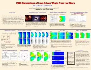
t=0 ksec 10 25 50 100 450 1 Ori C (O7 V) but for O-stars, to get h *~1, need: Bpole ~ 150 G forQ1Ori C ~300 G for ZPup Latitudinal Velocity X-ray Emission -12 -14 *=10 *=10 *=1 2.1 107 K 1.1 106 K 1 erg/cm3/s 0.1 erg/cm3/s Asif ud-Doula* & Stan Owocki MHD Simulations of Line-Driven Winds from Hot Stars Bartol Research Institute, University of Delaware, Newark, DE * NASA Space Grant College Fellow Pneuman and Kopp Model of Solar Corona Magnetically Confined Wind-Shocks (MCWS) Magnetic Effects on Solar Coronal Expansion Hot-Star Winds Babel & Montmerle 1997a,b MHD model for base dipole with Bo=1 G Our Simulation Magnetic Ap-Bp stars 1991 Solar Eclipse • Over the course of their lifetimes, hot, luminous, massive (OB-type) stars lose large amount of mass in nearly continous outflow called a stellar wind. • These winds are driven by scattering of the star’s continuum radiaton in a large ensemble of spectral lines (Castor, Abbott & Klein 1975; CAK) • There is extensive evidence for variability and structure on both small and large scales. • Our simulations show that magnetic fields may explain some of the large scale variability in wind flow, UV and X-ray emissions from hot stars. • There have been some positive detection of magnetic fields in hot stars, e.g, Donati et al. (2001) report a tilted dipole field of Bpole~300 G in Beta Ceph. Coronal streamers • At sunspot minimum, Sun has a global dipole magnetic field of about 1 Gauss. • Left panel: soft X-ray image of the sun; note dense, static closed loops. • Middle panel: solar corona; note coronal streamers where the wind opens field toward radial. • Right panel: solar wind outflow speed at 1 AU as a function of latitude. • Magnetic fields can modulate stellar winds. • First dynamical model of coronal streamers: Pneuman and Kopp (1971) using iterative scheme (left panel). • Dynamical MHD reproduction of this model using time explicit magnetohydrodynamic code (ZEUS-3D). • Effect of magnetic fields in hot stars: non-linear radiative force + MHD no simple analytical solutions. • Past attempts: fixed-field model of Babel and Montmerle (1997) to explain X-ray emission; flow computed along fixed magnetic flux tubes open-field outflow not modelled in detail. Fixed *( =10), Different Stars Inner Wind Relaxation of Wind to a Dipole Field Wind Magnetic Confinement Global Structure Log() (gm/cm3) Ratio of magnetic to kinetic energy density: for solar wind, h *~ 45 ... • Closed loops for * >1. • Magnetic flux tubes of opposite polarity guide wind outflow towards the magnetic equator wind collision heating of the gas (see below) X-ray. • Wind material stagnated after the shock: dense and slow radiative force inefficient gravity wins: infall of wind material in the form of dense knots onto the stellar surface. • Infall of dense knots: semi-regular, about every 200 ksec complex infall pattern. • Might explain red-shifted emission or absorption features (e.g., Smith et. al. 1991, ApJ 367, 302). Log of density and magnetic fields for three MHD models with same magnetic confinement parameter, *, but for three different stars: standard Pup, factor-ten lower mass loss rate Pup, and 1 Ori C. • Overall similarity: global configuration of field and flow depends mainly on the combination of stellar, wind, and magnetic properties that define *. • This dimensionless parameter, *is the governing parameter for our dynamical and self-consistentsimulations. • Assumptions: isothermal, non-rotating star. • Standard model: Pup (R=1.3 1012 cm, M=50 MSun, L=1.0 106 LSun, Mass loss=2.6 10-6 MSun/yr, Vinf=2300 km/s. Snapshots of density and magnetic field lines at the labeled time intervals starting from the initial condition of a dipole field superimposed upon a spherically symmetric outflow for *= sqrt(10) (Bpole=520G). • Comparison of density and magnetic field topology for different *, as noted. • Equatorial density enhancement for even * =1/10 • Wind always wins: field lines extended radially at the outer boundary for all cases Conclusion Mass Flux and Radial Outflow Velocity Velocity Modulation • Overall properties of the wind depend on *. • For *<1, the wind extends the surface magnetic field into an open, nearly radial configuration. • For *>1, the field remains closed in loops near the equatorial surface. Wind outflows from opposite polarity footpoints channeled by fields into strong collision near the magnetic equator can lead to hard X-ray emission. • For all cases, the more rapid radial decline of magnetic vs. wind-kinetic-energy density implies the field is eventually dominated by the wind, and extended into radial configuration. • Stagnated post-shock wind material falls back onto the stellar surface in a complex pattern. • These simulations may be relevant in interpreting various observational signatures of wind variability, e.g. UV line “Discrete Absorption Components”, X-ray emission. • Why is there a lot of hot gas outside the closed loops? • Slow radial speed within the disk high speed incoming material fully entrained with the disk big reduction of the speed high post-shock temperature. • See de Messieres et al., poster 135.12 for more on X-rays. • Radial mass flux density and radial flow speed at the outer boundary, r=6R*, normalized by values of the corresponding non-magnetic model, for the final time snapshot (t=450 ksec). • The horizontal dashed lines mark the unit values for the non-magnetic case. • Note: decrease of mass loss rate for * >1 • Radial outflow velocity for the case * =1 plotted as a function of latitude. • Can magnetic fields shape Planetary Nebulae? See Dwarkadas, poster 135.09 • Latitudinal velocities (V) for * =1,sqrt(10),10 models. • Classically, these velocities determine the hardness of X-ray emission. • We find: oblique shocks are very important in X-ray emission as well. (see next figure) For the strong magnetic confinement case (* =10), log of density superimposed with field lines, estimated shock temperature and X-ray emission above 0.1 keV (see preprint ud-Doula & Owocki 2002 for details). This work was supported by the NASA Space Grant College program at the University of Delaware, by NASA grants NAG5-3530 and NAG-11095, and by NSF grant AST-0097983.