Two-Variable Regression Model Overview
290 likes | 746 Vues
Learn the method of ordinary least square (OLS) for regression analysis. Understand assumptions and properties of OLS, Gauss-Markov Theorem, and coefficient of determination.

Two-Variable Regression Model Overview
E N D
Presentation Transcript
Two-Variable Regression Model: The problem of Estimation Unit 3
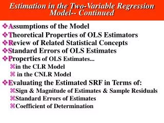
We will cover the following: • Method of ordinary least square (OLS) • Estimation of OLS regression parameters • Classical linear regression model: Assumptions underlying the model of OLS • Properties of least square estimators: Gauss-Markov Theorem • Coefficient of determination
The method of OLS The method of ordinary least squares is attributed to Carl Friedrich Gauss,a German mathematician. Under certain assumptions which we will discuss later, the method of least squares has some very attractive statistical properties that have made it one of the most powerful and popular methods of regression analysis. To understand this method, we first explain the least squares principle.
The method of OLS Recall the two-variable PRF: However, as we noted in the last unit, the PRF is not directly observable. We estimated from the SRF where is the estimated conditional mean of
The method of OLS • But how is the SRF itself determined? To see this, let us proceed as follows. which shows that the (the residuals) are simply the differences betweenthe actual and estimated Y values.
The method of OLS Now given n pairs of observations on Y and X, we would like to determine the SRF in such a manner that it is as close as possible to the actual Y. To this end, we may adopt the following criterion: Choose the SRF in such a way that the sum of the residuals is as small as possible but remember that summation of residuals is almost equal to zero. . We can avoid this problem if we adopt the least-squares criterion, which states that the SRF can be fixed in such a way that the SRF can be fixed in such a way that is as small as possible, where are the square residuals.
The method of OLS Let us differentiate with respect to and + + These are normal equations
The Classical Linear Regression Model: The Assumptions underlying the method of least square If our objective is to estimate β1 and β2 only, the method of OLS discussed in the preceding section will suffice. But recall from previous chapter that in regression analysis our objective is not only to obtainand but also to draw inferences about the true β1 and β2. For example, we would like to know how close and are to their counterparts in the population or how close is to the true E(Y | Xi). To that end, we must not only specify the functional form of the model but also make certain assumptions aboutthe manner in which Yi are generated.
The Classical Linear Regression Model: The Assumptions underlying the method of least square To see why this requirement is needed, look at the PRF: Yi = β1 + β2 Xi + ui . It shows that Yi depends on both Xi and ui . Therefore, unless we are specific about how Xi and ui are created or generated, there is no way we can make any statistical inference about the Yi and also, as we shall see, about β1 and β2 . Thus, the assumptions made about the Xi variable(s) and the error term are extremely critical to the valid interpretation of the regression estimates.
The Classical Linear Regression Model: The Assumptions underlying the method of least square TheGaussian,standard,orclassicallinearregressionmodel(CLRM), whichisthe cornerstoneof mosteconometrictheory,makes7assumptions. 1. Assumption 1: Linear regression model. The regression model is linear in the parameters Yi = β1 + β2Xi + ui
The Classical Linear Regression Model: The Assumptions underlying the method of least square 2. Assumption 2: X values are fixed in repeated sampling. Values taken by the regressor X are considered fixed in repeated samples. More technically, X is assumed to be nonstochastic 3. Assumption 3: Zero mean value of disturbance ui. Given the value of X, the mean, or expected, value of the random disturbance term ui is zero. Technically, the conditional mean value of ui is zero. Symbolically, we have E(ui |Xi) = 0
The Classical Linear Regression Model: The Assumptions underlying the method of least square
The Classical Linear Regression Model: The Assumptions underlying the method of least square
The Classical Linear Regression Model: The Assumptions underlying the method of least square Eq. (3.2.2) states that the variance of ui for each Xi (i.e., the conditional variance of ui ) is some positive constant number equal to σ 2 . Technically, (3.2.2) represents the assumption of homoscedasticity, or equal (homo) spread (scedasticity) or equal variance.. Put simply, the variation around the regression line (which is the line of average relationship between Y and X ) is the same across the X values; it neither increases or decreases as X varies.
The Classical Linear Regression Model: The Assumptions underlying the method of least square Diagrammatically, the situation is as depicted in Figure 3.4.
The Classical Linear Regression Model: The Assumptions underlying the method of least square
The Classical Linear Regression Model: The Assumptions underlying the method of least square
The Classical Linear Regression Model: The Assumptions underlying the method of least square In words, (3.2.5) postulates that the disturbances ui and uj are uncorre- lated. Technically, this is the assumption of no serial correlation, or no autocorrelation. This means that, given Xi , the deviations of any two Y val- ues from their mean value do not exhibit patterns such as those shown in Figure 3.6a and b. In Figure 3.6a, we see that the u’s are positively corre- lated, a positive u followed by a positive u or a negative u followed by a negative u. In Figure 3.6b, the u’s are negatively correlated, a positive u followed by a negative u and vice versa.
The Classical Linear Regression Model: The Assumptions underlying the method of least square
The Classical Linear Regression Model: The Assumptions underlying the method of least square • Assumption 6 states that the disturbance u and explanatory variable X are uncorrelated. The rationale for this assumption is as follows: When we expressed the PRF as in (2.4.2), we assumed that X and u (which may rep- resent the influence of all the omitted variables) have separate (and additive) influence on Y. But if X and u are correlated, it is not possible to assess their individual effects on Y. Thus, if X and u are positively correlated, X increases
The Classical Linear Regression Model: The Assumptions underlying the method of least square • Assumption 7: The number of observations n must be greater than the number of parameters to be estimated. Alternatively, the number of observations n must be greater than the number of explanatory variables. • This assumption is not so innocuous as it seems. In the hypothetical example of Table 3.1, imagine that we had only the first pair of observations on Y and X (4 and 1). From this single observation there is no way to esti- mate the two unknowns, β1 and β2 . We need at least two pairs of observa- tions to estimate the two unknowns. In a later chapter we will see the criti- cal importance of this assumption.
Properties of Least-Square Estimators: The Gauss-Markov Theorem As noted earlier, given the assumptions of the classical linear regression model, the least-squares estimates possess some ideal or optimum proper- ties. These properties are contained in the well-known Gauss–Markov theorem. To understand this theorem, we need to consider the best linear unbiasedness property of an estimator.
Properties of Least-Square Estimators: The Gauss-Markov Theorem An estimator, say the OLS estimator , is said to be a best linear unbiased estimator (BLUE) of if the following hold: 1. It is linear, that is, a linear function of a random variable, such as the dependent variable Y in the regression model. • It is unbiased, that is, its average or expected value, E(), is equal to the true value, β2 . 3. It has minimum variance in the class of all such linear unbiased estimators; an unbiased estimator with the least variance is known as an efficient estimator.
The coefficient of determination : A measure of goodness of fit
