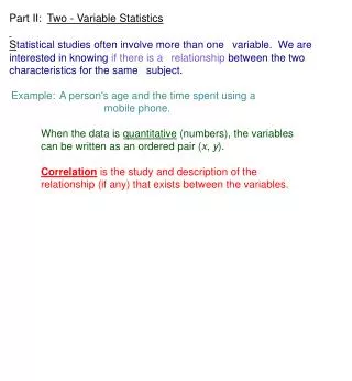
Correlation in Two-Variable Statistics
Learn how to interpret scatterplots, calculate correlation coefficient, and use regression modeling to understand relationships between variables. Correlation does not imply causation; additional analysis is needed to establish causality. Explore the methods of linear modeling to find best fit lines and regression equations. Estimate correlation coefficient and regression lines using a graphing calculator. Practice with in-class assignments on correlation and linear regression.

Correlation in Two-Variable Statistics
E N D
Presentation Transcript
Two-Variable Statistics Day 3: Linear Modeling
Warm-Up • Tell whether the data has a strong positive, weak positive, strong negative, or weak negative correlation. 2) 3) 1) 4) 5)
Interpreting scatterplots Look for overall pattern and deviations from the pattern. Describe overall pattern by form and strength (patterns closer to a straight line have more strength.) Outliers- a value that falls outside the overall pattern of the relationship. Positive or Negative association
Correlation Coefficient • Measures the strength of a linear relationship between a line and two variables. • Denoted as “r” • The r ranges from -1 to 1, where • r = 1 is a strong positive correlation • r = -1 is a strong negative correlation • r = 0.5 is a weak positive correlation • r = -0.5 is a weak negative correlation • r = 0 is no correlation
Correlation is NOT Causation • Just because two variables are highly correlated does NOT mean that one caused the other. • In order to prove causation, additional statistical analysis needs to occur. • For example, cigarette smoking and lung cancer are highly correlated, but additional studies were performed that actually PROVED that smoking cigarettes CAUSES lung cancer. • What did you learn from last night’s homework about the pirates on the high seas and the rising temp?
Finding the Correlation Coefficient • The calculation to compute r is complex. • For our purposes, we will estimate the correlation coefficient or use our graphing calculator to compute it for us. • Estimating the correlation coefficient: http://istics.net/stat/Correlations/
Using the Calculator Your graphing calculator uses the correlation coefficient to calculate the least squares regression line. To display the correlation coefficient r on your calculator: 1. Select Catalog ([2nd][0]) 2. Scroll down to place the pointer on “Diagnostics On” and press [ENTER] [ENTER] 3. Press [STAT], “Calc”, “4 LinReg ax+b” 4. The correlation coefficient, r, is displayed with the data for the regression line
Regression • The process of plotting data points and deriving an equation to model the data. • The function used to model the data is called the regression equation. • The graph of the linear equation is the regression line.
3 Methods of Linear Modeling 1. Best Fit Line / “Eyeballing” 2. Median-Median Line 3. Linear Regression (Least Squares Regression Line) The 3rd method is the most commonly used method to calculate a regression line.
Least Squares Regression Line (Called “LinReg” Line on Calc.) • A straight line that approximates the relationship between 2 variables • The Least Squares Regression calculation uses the sum of the squares of the vertical distances between each data point and a possible regression line. • You will not need to calculate this by hand! We will only use our graphing calculator to calculate the Least Squares Regression Line.
Using the Calculator • 1. Select [STAT] [EDIT] enter 2 lists of data • 2. Be sure that “Stat Plot” is turned ON and the “scatter plot” is selected • 3. To display the linear regression using the Least Squares Regression Line, Press [STAT] “Calc” • 4. Select “4. LinReg ax+b” The calculator will display the equation for the LSRL and the correlation coefficient (assuming you’ve set up your calculator correctly).
Today’s In Class Assignment Correlation Scatterplot Teenage Drinking and Driving Activity
Why the LSRL Model? • It more closely reflects the exact data points than either “eyeballing” (drawing a Best Fit Line) or calculating the Median-Median Line. • However, the Median-Median Line method is more resistant to outliers than the least squares regression line. So, if your data set includes outliers, the Median-Median Line method may give you a more accurate linear regression line.