On the use of eddy-covariance and optical remote sensing data for biogeochemical modelling

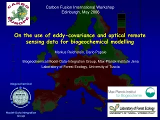
1. Biogeochemical Model-Data Integration Group Carbon Fusion International Workshop Edinburgh, May 2006 On the use of eddy-covariance and optical remote sensing data for biogeochemical modelling Markus Reichstein, Dario Papale Biogeochemical Model-Data-Integration Group, Max-Planck-Institute Jena Laboratory of Forest Ecology, University of Tuscia

2. BGC-Model-Data Integration Overview Ecosystem models + provide system understanding+ promise inter-/extrapolation capacity+ may include historical effects – are simplifications of the world– can’t predict stochastic events Ecosystem data Remote sensing + Potentially high quality+ often high temporal resolution – data compatibility ? – ‘point’ observations + objective/consistent observations+ spatially and temporally dense – data quality lower– processes not directly observable, no history, no prediction

3. Outline • Introduction to eddy covariance data • Bottom-up perspective of an ‘ideal’ data integration-validation process • Problems and obstacles in this process

4. Observing ecosystem gas exchange: eddy covariance Flux = speed x concentration Photo: Baldocchi

5. CO2, H2O Eddy covariance + Measures whole ecosystem exchange of CO2 and H2O, … + Non-destructive & continuous + time-scale hourly to interannual + integrates over large area - only on flat sites - relies on turbulent conditions ==> data gaps, stochastic data - source area varying (flux footprint) - only ‚point‘ measurements Does not deliver compartment fluxes, but: NEP = GPP - Reco

6. Respiration Carbon uptake Half-hourly eddy covariance data Evapotransp.

7. Raw data Knowledge 1013  108  106  102 bytes Model param. Synth./aggr. Turb stat. Network of ecosystem-level observations >1000 site-years  1012 raw measurements (1013 bytes) • Network and intercomparison studies • Harmonised and documented data processing • Aubinet et al. (2000), Falge et al. (2001), Foken et al. (2002), Göckede/Rebmann/Foken (2004) : general set-up and methodology, quality assurance, gap-filling • Reichstein et al. (2005), Glob. Ch. Biol.: u*-correction, gap-filling, partitioning of NEE • Papale et al. (in prep), Biogeosciences: Quality control, eval. uncertainties • Moffat et al. (in prep): Gap-filling inter-comparison • Online processing tool: http://gaia.agraria.unitus.it/lab/reichstein/

8. Model application Model(re)formulation(Definition of model structure) Model characterization(Forward runs, consistency check, sensitivity, uncert. analysis) Model validation (against indep. data, by scale or quantity) DATA Model parameter estimation(Multiple constraint) Generalization(‘up-scaling’) Parameterinterpretation(Thinking) Ideal model-data integration cycle (bottom-up)

9. Solar radiation Air temperature [CO2] Relative humidity Wind speed {Quantum use efficiency,electron transport and carboxylation capacities, stomatal conductance} LAI, SAI Canopy Layer 1 Canopy Layer 2 Phenology Canopy Layer 3 . . . Leaf Canopy Layer n physiology Canopy effective soil CO2 H2O CO2 Vapour pressure H2O Water extraction Precipitation Air temperature Wind speed Soil hydraulicparameters T, q, Y Soil thermalparameters Soil Layer 1 Soil Layer 2 Soil Layer 3 Soil respirationparameters T, q, Y . . . Soil Layer n Root distri-bution Soil The bottom-up model PROXEL

10. I. Model charaterization / forward model run Well watered conditions 0.2 Eddy cov. (a) (b) 0.18 Sap flow 0.16 Modelled 0.14 0.12 H2O flux [mm/h] 0.1 0.08 0.06 0.04 0.02 0 Eddy cov. (c) (d) 12 Modelled 10 8 6 CO2 flux of GPP [µmol m-2 s-1] 4 2 0 -2 0 4 8 12 16 20 24 0 4 8 12 16 20 24 Local time [hr] Local time [hr] Drought stressed conditions Reichstein, Tenhunen et al., Global Change Biology, 2002

11. Target region II. Dual-constraint parameter estimation Reichstein et al. 2003, JGR

12. IIa. Inferred parameter timeseries

13. III. Interpretation & Generalization Relative leaf activity Relative soil water content Reichstein et al. 2003, JGR

14. 1.8 1.6 III. Interpretation and Generalization: Keyp. RUEmax 1.4 1.2 1 RUE [gC / MJ APAR] 0.8 0.6 • inter-PFT variability • intra-PFT variability • f(species, N, T???) 0.4 0.2 0 ENF EBF DBF MF Sav Oshrub Crop

15. 29,2° W 58° E 70°N 60°N "Les Landes" 50°N 40°N 11° W 23° E IV. Validation at larger scale

16. GCB, in press

17. The problems

18. To consider with DA of eddy covariance data: • How is the error structure of the data itself? • How to address mismatch of scales (‘point’ versus pixel)? • Remote sensing • Meteorological data • How do perform up-scaling from tower sites? • Representativity • Generalization

19. Errors in the data

20. Error model influence on parameter estimates Search strategy I II Parameter estimate Const. abs errors Const. rel. errors Simplified after Trudinger et al. (OPTIC)

21. Errors in eddy covariance data • Random errors • ~ 30% for the half-hourly flux, (turbulences !) • Systematic errors • can be largely controlled/avoided • Selective systematic errors • Conditions where the theory does not apply: • Low turbulent conditions (night-time) • Advection • good quality control necessary • “Better few unbiased data, than a lot of biased data” • Uncertainties: mean NEE > interannual variability

22. Characterization of the random error cf. Richardson et al. (2006)

23. NEE [µmol m-2 s-1] 20.0 20 15 10 5 0 -5 -10 -13.0 15.00 14 12 10 8 6 4 2 0.00 Quantifying uncertainties NEE NEE_sigma Dec Dec Dec Dec Nov Nov Nov Nov Oct Oct Oct Oct Sep Sep Sep Sep Aug Aug Aug Aug Jul Jul Jul Jul NEE_sigma [µmol m-2 s-1] Jun Jun Jun Jun May May May Apr Apr Apr Apr Mar Mar Mar Mar Feb Feb Feb Feb Jan Jan Jan Jan 0 0 6 6 12 12 18 18 24 24 0 0 6 6 12 12 18 18 24 24

24. 3133 0.40 0.30 1401 0.20 1286 0.10 371 329 168 115 75 66 44 39 39 31 20 20 15 11 10 9 1 0 3 6 3 5 5 1 1 0 0.00 -20.0 -16.9 -13.8 -10.8 -7.7 -4.6 -1.5 1.5 4.6 7.7 10.8 13.8 16.9 20.0 Error NEE [umol m-2 s-1] Error distribution of eddy covariance data

25. Distribution of model error against eddy data Chevalier et al. (in rev.)

26. PDF only 10am-3pm and Jun-Sep NEE error

27. More complicated error structures

28. Maximizing the likelihood? Bayesian approach Cost function: Trust in data Trust in apriori model parameters

29. Spatial representation problem I • Does the tower site represent the grid cell of interest? • 0.25-2km km for MODIS/SEAWIFS remote sensing • 30-100 km for meteorological fields • 30-100 km for DGVMs, BGCs applied in global context

30. Aerial photo Landsat MODIS Spatial heterogeneity... 1 km

31. It‘s not always so bad... TM3 coeff. of variation • TM 3,4,7 • MODIS 1,2,7 Dinh et al., subm.

32. Spatial representation problem II • Does the network of tower sites represent the spatial domain of interest or are there chances to generalize with scaling variables?

33. fAPAR [MODIS-RT)  We have to have up-scaling strategies Day of the year

34. Conclusions • Eddy covariance data contains a lot of interpretable information on both carbon and water cycle • Inclusion of pools and fluxes for system understanding and for linking short and long time-scales necessary • Major challenge within eddy data • Characterization of the error (random, bias) • Scale and representativeness problem • Interpret. & Generalization of site specific parameters • Documentation of site dynamics, that may violate model structure (e.g., soil water, management)

35. Conclusions