Download
1 / 20
200 likes | 344 Vues
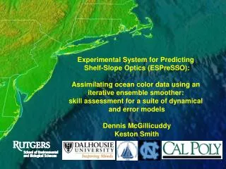
Experimental System for Predicting Shelf-Slope Optics (ESPreSSO): Assimilating ocean color data using an iterative ensemble smoother: skill assessment for a suite of dynamical and error models Dennis McGillicuddy Keston Smith.

E N D
Experimental System for Predicting Shelf-Slope Optics (ESPreSSO): Assimilating ocean color data using an iterative ensemble smoother: skill assessment for a suite of dynamical and error models Dennis McGillicuddy Keston Smith
Ocean color assimilation as a solution to the cloudiness problem State estimation (compositing) Process studies SW06 data – Gawarkiewicz et al.
Methodology Forward model (2-D): c: surface layer (20m) chlorophyll concentration v: velocity provided by hydrodynamic model D: diffusivity, 10 m s-2 S(x,y), R(x,y): unknown source/sink terms Data (d): H: linear measurement operator η: measurement error Approach: Utilize an ensemble (N=400) of Monte Carlo simulations to estimate initial conditions c(t0) and source/sink terms S(x,y),R(x,y)
Methodology cont’d Best prior estimate: Initialize with (climatology) Source/sink term S(x,y)=0; R(x,y)=0 Posterior estimates of the ICs and source sink terms are Gaussian perturbations about the best prior estimates of ci(t0),S(x,y), and R(x,y) lead to an ensemble of simulations Kalman gain computed from Monte Carlo approximations to the covariance between the unknown parameters and the model prediction of the observations
Use of an explicit biological model Nutrients: Phytoplankton: Satellite ocean color data samples the phytoplankton field:
Model domains Region of interest Assimilation subdomain Shelf-scale ROMS (9km resolution) He and Chen, submitted
Mean of the prior initial conditions: MODIS climatology for August Chlorophyll a – mg m-3
Results Ernesto Satellite data Prior RHS=0 RHS=S(x,y) RHS=R(x,y)c N-P model
Inferred biological fields RHS=S(x,y) RHS=R(x,y)c N-P model Uptake Mortality
Skill assessment: sensitivity to observational error RMS misfit to unassimilated data ADR 43% ADS 36% NP 32% AD 18% Observational error standard deviation
Comparisons with Gawarkiewicz in situ data Model vs. satellite Satellite vs. in situ Correlation Model vs. in situ Ernesto Year Day
Conclusions Ensemble smoothing methodology shows promise Goodness of fit depends on data (amount, underlying phenomenology) parameters of the assimilation procedure λx, λobs, σobs biological dynamics of the forward model Future directions apply to additional ESPreSSO / BIOSPACE field foci in situ data higher resolution time-dependent velocity fields methodological development more sophisticated bio-optical models joint uncertainties in physics and biology skill assessment
Sensitivity to observational error: misfit Prior misfit RMS misfit to active data Observational error standard deviation σobs=0.1
Methodology (3) Posterior estimates of the ICs and source sink terms are Kalman gain computed from observational error covariance W and the ensemble covariances P, Pc, and PR with
Methodology (4) Model prediction covariance (prior) Nobs X Nobs Monte Carlo approximations to the covariance between the unknown parameters and the model prediction of the observations: Nunk X Nobs
Methodology cont’d Best prior estimate: Initialize with (climatology) Source/sink term S(x,y)=0; R(x,y)=0 Gaussian perturbations about the best prior estimates of ci(t0),S(x,y), and R(x,y) lead to an ensemble of simulations Posterior estimates of the ICs and source sink terms are Kalman gain computed from Monte Carlo approximations to the covariance between the unknown parameters and the model prediction of the observations