Signature

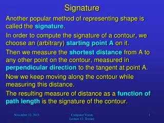
1. Signature • Another popular method of representing shape is called the signature. • In order to compute the signature of a contour, we choose an (arbitrary) starting point A on it. • Then we measure the shortest distance from A to any other point on the contour, measured in perpendicular direction to the tangent at point A. • Now we keep moving along the contour while measuring this distance. • The resulting measure of distance as a function of path length is the signature of the contour. Computer Vision Lecture 12: Texture

2. Signature • Notice that if you normalize the path length, the signature representation is position, rotation, and scale invariant. • Smoothing of the contour before computing its signature may be necessary for a useful computation of the tangent. Computer Vision Lecture 12: Texture

3. Fourier Transform of Boundaries • As we discussed before, a 2D contour can be represented by two 1D functions of a parameter s. • Let S be our (arbitrary) starting point on the contour. • By definition, we should move in counterclockwise direction (for example, we can adapt the boundary-following algorithm to do that). • In our discrete (pixel) space, the points of the contour can then be specified by [v[s], h[s]], • where s is the distance from S (measured along the contour) • and v and h are the functions describing our vertical and horizontal position on the contour for a given s. Computer Vision Lecture 12: Texture

4. Fourier Transform of Boundaries Computer Vision Lecture 12: Texture

5. Fourier Transform of Boundaries Computer Vision Lecture 12: Texture

6. Fourier Transform of Boundaries • Obviously, both v[s] and h[s] are periodic functions, as we will pass the same points over and over again in constant time intervals. • This gives us a brilliant idea: Why not represent the contour in Fourier space? • In fact, this can be done. We simply compute separate 1D Fourier transforms for v[s] and h[s]. • When we convert the result into the magnitude/phase representation, the transform gives us the functions • Mv[l],Mh[l],v[l],and h[l] • for frequency l ranging from 0 (offset) to s/2. Computer Vision Lecture 12: Texture

7. Fourier Transform of Boundaries • As with images, higher frequencies do not usually contribute much to a function an can be disregarded without any noticeable consequences. • Let us see what happens when we delete all functions above frequency lmax and perform the inverse Fourier transform. • Will the original contour be conserved even for small values of lmax? Computer Vision Lecture 12: Texture

8. Fourier Transform of Boundaries Computer Vision Lecture 12: Texture

9. Fourier Transform of Boundaries Computer Vision Lecture 12: Texture

10. Fourier Transform of Boundaries • The phase spectrum of the Fourier description usually depends on our chosen starting point. • The power (magnitude) spectrum, however, is invariant to this choice if we combine vertical and horizontal magnitude as follows: • We can cut off higher-frequency descriptors and still have a precise and compact contour representation. • If we normalize the values of all M[l] so that they add up to 1, we obtain scale-invariant descriptors. Computer Vision Lecture 12: Texture

11. Computer Vision Lecture 12: Texture

12. Our next topic is… • Texture Computer Vision Lecture 12: Texture

13. Texture Computer Vision Lecture 12: Texture

14. Texture • Texture is an important cue for biological vision systems to estimate the boundaries of objects. • Also, texture gradient is used to estimate the orientation of surfaces. • For example, on a perfect lawn the grass texture is the same everywhere. • However, the further away we look, the finer this texture becomes – this change is called texture gradient. • For the same reasons, texture is also a useful feature for computer vision systems. Computer Vision Lecture 12: Texture

15. Texture Gradient Computer Vision Lecture 12: Texture

16. Texture • The most fundamental question is: How can we “measure” texture, i.e., how can we quantitatively distinguish between different textures? • Of course it is not enough to look at the intensity of individual pixels. • Since the repetitive local arrangement of intensity determines the texture, we have to analyze neighborhoods of pixels to measure texture properties. Computer Vision Lecture 12: Texture

17. Frequency Descriptors • One possible approach is to perform local Fourier transforms of the image. • Then we can derive information on • the contribution of different spatial frequencies and • the dominant orientation(s) in the local texture. • For both kinds of information, only the power (magnitude) spectrum needs to be analyzed. Computer Vision Lecture 12: Texture

18. Frequency Descriptors • Prior to the Fourier transform, apply a Gaussian filter to avoid horizontal and vertical “phantom” lines. • In the power spectrum, use ring filters of different radii to extract the frequency band contributions. • Also in the power spectrum, apply wedge filters at different angles to obtain the information on dominant orientation of edges in the texture. Computer Vision Lecture 12: Texture

19. Frequency Descriptors • The resulting frequency and orientation data can be normalized, for example, so that the sum across frequency or orientation bands is 1. • This effectively turns them into histograms that are less affected by monotonic gray-level changes caused by shading etc. • However, it is recommended to combine frequency-based approaches with space-based approaches. Computer Vision Lecture 12: Texture

20. Co-Occurrence Matrices • A simple and popular method for this kind of analysis is the computation of gray-level co-occurrence matrices. • To compute such a matrix, we first separate the intensity in the image into a small number of different levels. • For example, by dividing the usual brightness values ranging from 0 to 255 by 64, we create the levels 0, 1, 2, and 3. Computer Vision Lecture 12: Texture

21. Co-Occurrence Matrices • Then we choose a displacement vectord = [di, dj]. • The gray-level co-occurrence matrix P(a, b) is then obtained by counting all pairs of pixels separated by d having gray levels a and b. • Afterwards, to normalize the matrix, we determine the sum across all entries and divide each entry by this sum. • This co-occurrence matrix contains important information about the texture in the examined area of the image. Computer Vision Lecture 12: Texture

22. 0 1 0 0 1 0 0 1 1 1 0 1 1 0 0 0 1 0 0 1 0 1 1 1 0 1 1 0 0 1 0 0 1 0 d = (1, 1) 1 1 0 1 1 0 local texture patch displacement vector co-occurrence matrix Co-Occurrence Matrices • Example (2 gray levels): 2 9 1/25  10 4 Computer Vision Lecture 12: Texture

23. Co-Occurrence Matrices • It is often a good idea to use more than one displacement vector, resulting in multiple co-occurrence matrices. • The more similar the matrices of two textures are, the more similar are usually the textures themselves. • This means that the difference between corresponding elements of these matrices can be taken as a similarity measure for textures. • Based on such measures we can use texture information to enhance the detection of regions and contours in images. Computer Vision Lecture 12: Texture

24. Co-Occurrence Matrices • For a given co-occurrence matrix P(a, b), we can compute the following six important characteristics: Computer Vision Lecture 12: Texture

25. Co-Occurrence Matrices Computer Vision Lecture 12: Texture

26. Co-Occurrence Matrices • You should compute these six characteristics for multiple displacement vectors, including different directions. • For example, you could use the following vectors: • (-3, 0), (-2, 0), (-1, 0) (1, 0), (2, 0), (3, 0) • (0, -3), (0, -2), (0, -1) (0, 1), (0, 2), (0, 3) • (-3, -3), (-2, -2), (-1, -1) (1, 1), (2, 2), (3, 3) • (-3, 3), (-2, 2), (-1, 1) (1, -1), (2, -2), (3, -3) • The maximum length of your displacement vectors depend on the size of the texture elements. Computer Vision Lecture 12: Texture

27. Law’s Texture Energy Measures • Law’s measures use a set of convolution filters to assess gray level, edges, spots, ripples, and waves in textures. • This method starts with three basic filters: • averaging: L3 = (1, 2, 1) • first derivative (edges): E3 = (-1, 0, 1) • second derivative (curvature): S3 = (-1, 2, -1) Computer Vision Lecture 12: Texture

28. Law’s Texture Energy Measures • Convolving these filters with themselves and each other results in five new filters: • L5 = (1, 4, 6, 4, 1) • E5 = (-1, -2, 0, 2, 1) • S5 = (-1, 0, 2, 0, -1) • R5 = (1, -4, 6, -4, 1) • S5 = (-1, 2, 0, -2, 1) Computer Vision Lecture 12: Texture

29. Law’s Texture Energy Measures • Now we can multiply any two of these vectors, using the first one as a column vector and the second one as a row vector, resulting in 5  5 Law’s masks. • For example: Computer Vision Lecture 12: Texture

30. Law’s Texture Energy Measures • Now you can apply the resulting 25 convolution filters to a given image. • The 25 resulting values at each position in the image are useful descriptors of the local texture. • Law’s texture energy measures are easy to apply and give good results for most texture types. • However, co-occurrence matrices are more flexible; for example, they can be scaled to account for coarse-grained textures. Computer Vision Lecture 12: Texture

31. Co-Occurrence Matrices • Benchmark image for texture segmentation – an ideal segmentation algorithm would divide this image into five segments. • For example, a texture-descriptor based variant of split-and-merge may be able to achieve good results. Computer Vision Lecture 12: Texture