Aggregate Demand I
Aggregate Demand I. The Economy in the Short-run. Introduction. Here, we continue our study of economic fluctuations by looking more deeply at aggregate demand In the long-run prices are flexible and aggregate supply determines income

Aggregate Demand I
E N D
Presentation Transcript
Aggregate Demand I The Economy in the Short-run Source: "Macroeconomics" , Mankiw, Fourth Edition: Chapter 10, Fifth Edition: Chapter 10
Introduction • Here, we continue our study of economic fluctuations by looking more deeply at aggregate demand • In the long-run prices are flexible and aggregate supply determines income • In the short-run, prices are sticky, so changes in aggregate demand influence income Source: "Macroeconomics" , Mankiw, Fourth Edition: Chapter 10, Fifth Edition: Chapter 10
Introduction • In 1936: John Maynard Keynes revolutionised economics with his book: The General Theory of Employment, Interest and Money • Keynes proposed that low aggregate demand is responsible for the low income and high unemployment that characterise economic downturns Source: "Macroeconomics" , Mankiw, Fourth Edition: Chapter 10, Fifth Edition: Chapter 10
Introduction • In previous chapter we derived the aggregate demand curve very simply using the quantity theory of money and we showed how monetary policy shifts the AD curve • This was an incomplete derivation of the AD curve • Here, we provide a complete derivation of the AD curve and show that fiscal and monetary policy will affect the AD curve Source: "Macroeconomics" , Mankiw, Fourth Edition: Chapter 10, Fifth Edition: Chapter 10
Introduction • The model to explain the AD curve is the IS-LM model • It is an interpretation of Keynes’ theory • IS: stands for investment and saving • IS curve represents what’s going on in the market for goods and services • LM: stands for liquidity and money • LM curve represents what’s going on in the money market (demand and supply of money) Source: "Macroeconomics" , Mankiw, Fourth Edition: Chapter 10, Fifth Edition: Chapter 10
Introduction • IS-LM Model: • Model of aggregate demand • It is based in the short-run, when prices are sticky • It shows what causes income to change and therefore what causes the aggregate demand curve to shift Source: "Macroeconomics" , Mankiw, Fourth Edition: Chapter 10, Fifth Edition: Chapter 10
Theory of Short-run Fluctuations Source: "Macroeconomics" , Mankiw, Fourth Edition: Chapter 10, Fifth Edition: Chapter 10
Summary • What we will cover in this topic (over 2 chapters): • Derive the IS curve using the Keynesian cross theory • Derive the LM curve using the Liquidity Preference theory • Put the IS-LM curves together (which maps interest rates and output) • Study how fiscal policy shifts the IS curve and monetary policy shifts the LM • Use the IS-LM model to derive the aggregate demand curve • Use the IS-LM model to show how monetary and fiscal policy shift the aggregate demand curve Source: "Macroeconomics" , Mankiw, Fourth Edition: Chapter 10, Fifth Edition: Chapter 10
The Goods Market and the IS Curve • IS curve: plots the relationship between the interest rate and the level of income that arises in the market for goods and services • To develop the relationship, we use a theory called: the Keynesian cross Source: "Macroeconomics" , Mankiw, Fourth Edition: Chapter 10, Fifth Edition: Chapter 10
The Goods Market and the IS Curve • Keynes proposed that in the short run, economy’s income depended largely on the desire to spend by households, firms and the government. • More people spend, more goods and services firms can sell, more output will be produced, more workers will be hired • Problem during economic recessions: inadequate spending • The Keynesian Cross models this proposal Source: "Macroeconomics" , Mankiw, Fourth Edition: Chapter 10, Fifth Edition: Chapter 10
The Goods Market and the IS Curve • The Keynesian Cross: • Distinction between actual and planned expenditure • Actual expenditure = amount households, firms and the government spend on goods and services • Planned expenditure = amount households, firms and the government would like to spend on goods and services Source: "Macroeconomics" , Mankiw, Fourth Edition: Chapter 10, Fifth Edition: Chapter 10
The Goods Market and the IS Curve • Keynesian Cross: • Why would actual and planned expenditure be different? • Answer: firms might engage in unplanned inventory investment if sales do not meet expectations. Firms sell less of the product than expected, stock of inventories rises. And if sales exceed expectations, stock of inventories falls. These unplanned changes in inventory are counted as investment spending by firms Source: "Macroeconomics" , Mankiw, Fourth Edition: Chapter 10, Fifth Edition: Chapter 10
The Goods Market and IS Curve • Keynesian cross: • Determinants of planned expenditure • Assume economy is closed (no exports or imports) • Planned expenditure (E) = sum of consumption (C), planned investment (I), and government purchases (G) E = C + I + G Source: "Macroeconomics" , Mankiw, Fourth Edition: Chapter 10, Fifth Edition: Chapter 10
The Goods Market and IS Curve • Keynesian cross: E = C + I + G : Planned expenditure • To this we add the consumption function: C = C(Y-T) • For now, assume planned investment is fixed I = I • Assume government purchases and taxes are fixed by the government (fixed fiscal policy) G = G T = T Source: "Macroeconomics" , Mankiw, Fourth Edition: Chapter 10, Fifth Edition: Chapter 10
The Goods Market and IS Curve • Keynesian cross: E = C(Y-T) + I + G • Planned expenditure is a function of income • Graph of planned expenditure • Upward sloping: higher income leads to higher expenditure (because higher income leads to higher consumption, which is part of planned expenditure) • Slope of the line is the marginal propensity to consume Source: "Macroeconomics" , Mankiw, Fourth Edition: Chapter 10, Fifth Edition: Chapter 10
Source: "Macroeconomics" , Mankiw, Fourth Edition: Chapter 10, Fifth Edition: Chapter 10
The Goods Market and the IS Curve • Keynesian Cross • Planned expenditure: first piece of Keynesian cross • Next piece of Keynesian cross: assumption that the economy is in equilibrium when actual expenditure equals planned expenditure: (when people’s plans have been realised, there is no need to change) • Recall: Y (GDP) = total income and total output and total expenditure on goods and services in economy Source: "Macroeconomics" , Mankiw, Fourth Edition: Chapter 10, Fifth Edition: Chapter 10
The Goods Market and the IS Curve • Keynesian Cross: • Equilibrium condition: Actual expenditure = Planned Expenditure Y = E • 45-degree line with Y on the horizontal axis and E on the vertical axis: shows all the points where the equilibrium condition holds • Every point on the 45-degree: actual expenditure equals planned expenditure • Graph: the Keynesian Cross Source: "Macroeconomics" , Mankiw, Fourth Edition: Chapter 10, Fifth Edition: Chapter 10
Source: "Macroeconomics" , Mankiw, Fourth Edition: Chapter 10, Fifth Edition: Chapter 10
The Goods Market and the IS Curve • Keynesian cross: • Point A: Equilibrium of the economy, where planned expenditure equals actual expenditure (where the planned expenditure function crosses the 45-degree line) • How does the economy get to that equilibrium? Source: "Macroeconomics" , Mankiw, Fourth Edition: Chapter 10, Fifth Edition: Chapter 10
Source: "Macroeconomics" , Mankiw, Fourth Edition: Chapter 10, Fifth Edition: Chapter 10
The Goods Market and the IS Curve • Keynesian cross: • Suppose GDP or output is at Y1 , then planned expenditure E1 is less than production Y1 : • firms are selling less than they are producing • Firms add the unsold goods to their stock of inventories • This induces firms to layoff workers and reduce production • So Y falls Source: "Macroeconomics" , Mankiw, Fourth Edition: Chapter 10, Fifth Edition: Chapter 10
The Goods Market and the IS Curve • Keynesian Cross: • Suppose GDP or output is at Y2 , then planned expenditure E2 is greater than production Y2 : • Firms are selling more than expected, so they draw from inventories • This induces firms to hire more workers and increase production • So Y increases Source: "Macroeconomics" , Mankiw, Fourth Edition: Chapter 10, Fifth Edition: Chapter 10
The Goods Market and the IS Curve • In Keynesian cross: given levels of planned Investment I and fiscal policy, G (government purchases) and T (taxes) • Use this to show how income changes when we change one of these exogenous variables • Government purchases: consider how changes in government purchases affect the economy Source: "Macroeconomics" , Mankiw, Fourth Edition: Chapter 10, Fifth Edition: Chapter 10
The Goods Market and the IS Curve • Keynesian Cross: E = C(Y-T) + I + G • Higher government purchases result in higher planned expenditure • If G changes by ΔG then the planned expenditure function shifts upward (see graph on next slide) • Equilibrium in the economy moves from point A to point B. Increase in G causes Y to increase Source: "Macroeconomics" , Mankiw, Fourth Edition: Chapter 10, Fifth Edition: Chapter 10
Source: "Macroeconomics" , Mankiw, Fourth Edition: Chapter 10, Fifth Edition: Chapter 10
The Goods Market and the IS Curve • Keynesian cross: (government-purchases multiplier) • The change in income is more than what the change in government purchases was • i.e. ∆Y is larger than ∆G • Ratio ∆Y/ ∆G is called the government-purchases multiplier: it tells us how much income rises in response to a €1 increase in government purchases • Keynesian cross: the government purchases multiplier is larger than 1 Source: "Macroeconomics" , Mankiw, Fourth Edition: Chapter 10, Fifth Edition: Chapter 10
The Goods Market and the IS Curve • Keynesian cross: (government-purchases multiplier) • Why does fiscal policy have a multiplier effect on income? • Answer relates to the consumption function: C = C(Y – T) • When government purchases increase, this raises income, Y (Remember Y = E = C + I + G). This increase in Y in turn increases consumption, C. Source: "Macroeconomics" , Mankiw, Fourth Edition: Chapter 10, Fifth Edition: Chapter 10
The Goods Market and the IS Curve • Keynesian cross: (government-purchases multiplier) (cont’d) • The increase in consumption, in turn, increases income again, which further increases consumption and so on. • How big is the multiplier? Source: "Macroeconomics" , Mankiw, Fourth Edition: Chapter 10, Fifth Edition: Chapter 10
The Goods Market and the IS Curve • Keynesian cross: (government-purchases multiplier) (cont’d) • Let’s trace through each step of the change in income: Initial change in G = ∆G, so Y (income) changes by ∆G as well. This increase in income raises consumption by MPC x ∆G, where MPC = Marginal Propensity to Consume (as income increases by €1 the MPC tells us how much consumption will increase by) Source: "Macroeconomics" , Mankiw, Fourth Edition: Chapter 10, Fifth Edition: Chapter 10
The Goods Market and the IS Curve • Keynesian cross: (government-purchases multiplier) (cont’d) • Tracing through each step of the change in income (cont’d): The increase in consumption raises income again, which raises consumption again and so on. • Using algebra, the government purchases multiplier is: ∆Y/ ∆G = 1/(1- MPC) Source: "Macroeconomics" , Mankiw, Fourth Edition: Chapter 10, Fifth Edition: Chapter 10
The Goods Market and the IS Curve • Keynesian cross: (government-purchases multiplier) (cont’d) • Example: MPC = 0.6 ∆Y/ ∆G = 1/(1- MPC) = 1/(1 – 0.6) = 2.5 This says that a €1 increase in government purchases will lead to a €2.50 increase in equilibrium income Source: "Macroeconomics" , Mankiw, Fourth Edition: Chapter 10, Fifth Edition: Chapter 10
The Goods Market and the IS Curve • Keynesian cross: • What if taxes change? E = C(Y – T) + I + G • A decrease in taxes raises disposable income (Y-T) and therefore increases consumption • Therefore, planned expenditure function shifts upward • Economy moves from equilibrium A to equilibrium B (See graph) Source: "Macroeconomics" , Mankiw, Fourth Edition: Chapter 10, Fifth Edition: Chapter 10
Source: "Macroeconomics" , Mankiw, Fourth Edition: Chapter 10, Fifth Edition: Chapter 10
The Goods Market and the IS Curve • Keynesian Cross: (tax multiplier) • Just as with an increase in government purchases, a decrease in taxes has a multiplied effect on income • A decrease in taxes by ∆T increases consumption by MPC x ∆T, which increases Y, which increases consumption and so on. Source: "Macroeconomics" , Mankiw, Fourth Edition: Chapter 10, Fifth Edition: Chapter 10
The Goods Market and the IS Curve • Keynesian Cross: (tax multiplier) • Using algebra the tax multiplier is ∆Y/ ∆T = - MPC/(1- MPC) • Example: MPC = 0.6 ∆Y/ ∆T = - 0.6/(1- 0.6) = -1.5 • This says that a €1 cut in taxes raises equilibrium income by €1.50 Source: "Macroeconomics" , Mankiw, Fourth Edition: Chapter 10, Fifth Edition: Chapter 10

