Regression
Regression. Weight. Height. What would you expect for other heights?. How much would an adult female weigh if she were 5 feet tall?. This distribution is normally distributed. (we hope).

Regression
E N D
Presentation Transcript
Weight Height What would you expect for other heights? How much would an adult female weigh if she were 5 feet tall? This distribution is normally distributed. (we hope) She could weigh varying amounts – in other words, there is a distribution of weights for adult females who are 5 feet tall. What about the standard deviations of all these normal distributions? We want the standard deviations of all these normal distributions to be the same. Where would you expect the TRUE LSRL to be?
Regression Model • The mean response μy has a straight-line relationship with x: • Where: slope β and intercept α are unknown parameters • For any fixed value of x, the responsey varies according to a normal distribution. Repeated responses of y are independent of each other. • The standard deviation of y (sy) is the same for all values of x. (sy is also an unknown parameter)
We use to estimate • The slope b of the LSRL is an unbiased estimator of the true slope β. • The intercept a of the LSRL is an unbiased estimator of the true intercept α. • The standard error s is an unbiased estimator of the true standard deviation of y (sy). Note: df = n-2
Weight Height Suppose you took many samples of the same size from this population & calculated the LSRL for each. Using the slope from each of these LSRLs – we can create a sampling distribution for the slope of the true LSRL. What is the standard deviation of the sampling distribution? What is the mean of the sampling distribution equal? What shape will this distribution have? b b b b b b b μb = b
Assumptions for inference on slope • The observations are independent • Check that you have an SRS • The true relationship is linear • Check the scatter plot & residual plot • The standard deviation of the response is constant. • Check the scatter plot & residual plot • The responses vary normally about the true regression line. • Check a histogram or boxplot of residuals
Formulas: • Confidence Interval: • Hypothesis test: df = n -2 Because there are two unknowns a & b
Hypotheses This implies that there is no relationship between x & y Or that x should not be used to predict y What would the slope equal if there were a perfect relationship between x & y? H0: β = 0 Ha: β > 0 Ha: β < 0 Ha: β ≠ 0 1 Be sure to define β!
Example: It is difficult to accurately determine a person’s body fat percentage without immersing him or her in water. Researchers hoping to find ways to make a good estimate immersed 20 male subjects, and then measured their weights. • Find the LSRL, correlation coefficient, and coefficient of determination. Body fat = -27.376 + 0.250 weight r = 0.697 r2 = 0.485
b) Explain the meaning of slope in the context of the problem. There is approxiamtely .25% increase in body fat for every pound increase in weight. c) Explain the meaning of the coefficient of determination in context. Approximately 48.5% of the variation in body fat can be explained by the regression of body fat on weight.
Body fat Residuals Weight Weight d) Estimate a, b, and s. α = -27.376 β = 0.25 s = 7.049 e) Create a scatter plot and residual plot for the data.
f) Is there sufficient evidence that weight can be used to predict body fat? • Assumptions: • Have an SRS of male subjects • Since the residual plot is randomly scattered, weight & body fat are linear • Since the points are evenly spaced across the LSRL on the scatterplot, sy is approximately equal for all values of weight • Since the boxplot of residual is approximately symmetrical, the responses are approximately normally distributed. • H0: β = 0 Where β is the true slope of the LSRL of weight Ha: β ≠ 0 & body fat • Since the p-value < α, I reject H0. There is sufficient evidence to suggest that weight can be used to predict body fat.
g) Give a 95% confidence interval for the true slope of the LSRL. • Assumptions: • Have an SRS of male subjects • Since the residual plot is randomly scattered, weight & body fat are linear • Since the points are evenly spaced across the LSRL on the scatterplot, sy is approximately equal for all values of weight • Since the boxplot of residual is approximately symmetrical, the responses are approximately normally distributed. • We are 95% confident that the true slope of the LSRL of weight & body fat is between 0.12 and 0.38. Be sure to show all graphs!
h) Here is the computer-generated result from the data: Sample size: 20 R-square = 43.83% s = 7.0491323 df? What does “s” represent (in context)? Correlation coeficient? Be sure to write as decimal first! What do these numbers represent? What does this number represent?

