BACKPROPAGATION (CONTINUED)
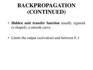
BACKPROPAGATION (CONTINUED). Hidden unit transfer function usually sigmoid (s-shaped), a smooth curve. Limits the output (activation) unit between 0..1. Take net input to unit, pass through function: gives output of unit. Most common is Logistic function:. Transfer function.

BACKPROPAGATION (CONTINUED)
E N D
Presentation Transcript
BACKPROPAGATION (CONTINUED) • Hidden unit transfer function usually sigmoid (s-shaped), a smooth curve. • Limits the output (activation) unit between 0..1
Take net input to unit, pass through function: gives output of unit. Most common is Logistic function:
Transfer function • Often use same function for output units (when building classifier, I.e. 0..1 classification) • For regression problems (decimal outputs) output transfer function used is linear (just sum net inputs)
Local minima • Backpropagation is a gradient descent process, each change in weights bringing net closer to a minimum error in weight space. • Because of this, easily trapped in local minimum, as only 'downward' steps can be taken. • Sometimes remedied by starting with different random weights (starting from different point in the error surface).
Critical parameters • Cumulative versus incremental weight changing. • Adjust weights after presentation of one pattern (incremental) or all (epoch)? • Epoch faster, but more likely to fall into local minima and requires more memory.
Critical parameters • Size of learning constant. • Too high – won’t learn anything (oscillate). Too low, will take ages to find solution.
Critical parameters • Momentum method. • Supplement current weight adjustments with a fraction of most recent weight adjustment.
Standard back-propagation weight adjustment: i.e. weight at time t+1 equal to weight at t plus (learning rate * calculated weight change).
Back propagation with momentum included, where alpha is momentum constant: i.e. we have included some of weight change from previous cycle of back-propagation. Can significantly speed up learning.
Critical parameters • Number of hidden units: • Too few, won’t learn problem. • Too many, network generalises poorly to new data (overfits training data).
Addition of Bias units • Bias is unit which always has output of 1, sometimes helps convergence of weights to an solution by providing extra degree of freedom in weight space.
Bias error derivatives (analogous to weight error derivatives in normal backprop) are calculated: i.e. the Bias error derivative for an output unit is found using the delta of that output unit multiplied by the output of the bias unit it connects to (i.e. 1).
In a similar way the Bias error derivatives for the hidden units are found:
Bias weights then changed in the same way as the other weights in the network, using the Bias error derivatives and a Bias change rate parameter beta ( analogous to n the learning rate parameter for normal weights):
In the same way, the Bias weights are changed for the hidden units:
Bias units • Bias units not mandatory but as they involve relatively little extra computation most neural networks have them by default.
Overtraining • Overtraining a type of overfitting • Can train network too much. • Network becomes very good at classifying the training set, but poor at classifying the test set that it has not encountered before, i.e. it is not generalising well (overfitting training data).
Overtraining • Avoid by periodically presenting a validation set and recording the error and storing weights. Best set of weights giving minimum error on the test set retrieved when training finished. • Some neural network packages do this for you, in a way that is hidden from the user.
Data selection • Selection of training data critical • When training to perform in a noisy environment must include noisy input patterns in the training set. • MLP good at interpolation but not at extrapolation. • Must balance number of members of each class in training and validation sets
Catastrophic forgetting • Unwise to train the network completely on patterns selected from one class and then switch to training from another class of patterns, as the network will forget the original training. • Solution is to mix both classes in same training set.