Download
1 / 21
210 likes | 318 Vues
This research focuses on accurate cell segmentation in microscopy images through a bag of local Bayesian classifiers. The system combines localized classifiers to assign probabilities to new pixels. Training involves spectral clustering and training of classifiers for improved segmentation results.

E N D
Cell Segmentation in Microscopy Imagery Using a Bag of Local Bayesian Classifiers Zhaozheng Yin RI/CMU, Fall 2009
Motivation • Accurate segmentation is challenging Segmentation using a single threshold yields poor results: Segmentation using a singe global Bayesian classifier also generates bad results:
Our Solution • A bag of local Bayesian classifiers: • Local Bayesian classifiers (experts) are learned from clustered training image patches. • Any new pixel to be classified is assigned a posterior probability about how likely it is a cell or background pixel based on the mixture-of-experts model.
System Overview Train and combine a bag of local Bayesian classifiers: Using the Bayes’ rule on each local Bayesian classifier, we have : where: is the feature around pixel x, for example, intensity, gradient etc. represents pixel class (Cell or Background ) is the weight dependent on the input (different from boosting) A new input pixel is classified by Maximum a Posteriori (MAP):
Training (get ) • Spectral clustering on local histograms (a) Compute local histograms around N sample pixels (b) Compute a pair-wise similarity matrix among the N histograms. (c) Group the N histograms into K clusters.
Training (get ) 2. Train local Bayesian classifiers (d) Achieve local histogram clusters from the spectral clustering (e) Obtain corresponding clustered image patches (f) Train local Bayesian classifiers from the clustered image patches
Classification • First , we calculate a local histogram around , and then compute the similarity between and every histogram cluster, , where represents the histogram of cluster . • The weighting function on classifier is defined as • We combine the local Bayesian classifiers as • Pixel is classified by
Classifier 2 Classifier 3 Classifier 1 h=5 win size h=10 h=15
Cyan square: miss detection Yellow circle: false alarm Red: our detection Green contour: ground truth
Cyan square: miss detection Yellow circle: false alarm Red: our detection Green contour: ground truth
Cyan square: miss detection Yellow circle: false alarm Red: our detection Green contour: ground truth
Cyan square: miss detection Yellow circle: false alarm Red: our detection Green contour: ground truth
Cyan square: miss detection Yellow circle: false alarm Red: our detection Green contour: ground truth
Input: Cell posterior probability: Ground truth labeling:
Bayesian Classifiers on DIC Images • We use intensity and gradient features on DIC images 10 bin Ix (intensity) 10 bin Gx (gradient magnitude)
Cluster k=1 k=2 k=3 Win sz h = 5 h = 10 h = 20
Conclusion • We propose a bag of local Bayesian classifier approach for cell segmentation in microscopy imagery. • Our approach is validated on four types of cells of different appearances captured by different imaging modalities and device settings with 92.5% average accuracy.