Download
1 / 39
390 likes | 416 Vues
Explore the impact of magneto-convection on solar irradiance variations using the MURaM code. Discover statistical and photometric properties, ranging from quiet Sun to strong plage. Learn about the structure, dynamics, and brightness relationships in solar magneto-convection simulations. Investigate applications, including photospheric flux concentrations and fractal dimensions of magnetic patterns. Gain insights into physical phenomena like G-band bright points and the origin of faculae brightening. This research sheds light on the complexities of solar activity and its influence on Earth's climate.

E N D
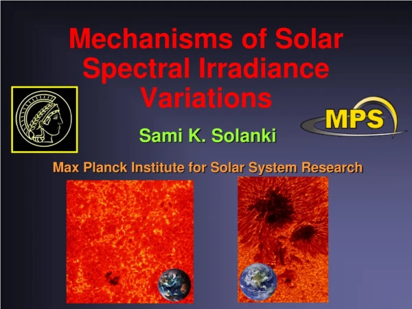
Solar Variability and Earth's Climate, Rome, June 29, 2005 Simulations of magneto-convection and solar irradiance variations A. Vögler, M. Schüssler, S.K. Solanki, V. Zakharov Max-Planck-Institute for Solar System Research
Outline • Introduction: magneto-convection and the MURaM code • Mechanisms: brightening of network points and faculae • Simulations: from „quiet“ Sun to strong plage • Results: Statistical & photometric properties • Summary
Regimes of solar magneto-convection • horizontal scale of convection decreases • convective energy transport decreases quiet Sun sunspot umbra plage average B sunspot umbra plage ‘quiet’ Sun G-band image: KIS/VTT, Obs. del Teide, Tenerife
The MPS/UofC Radiation MHD (MURaM) Code Developed by the MPS MHD group (A. Vögler, R. Cameron, S. Shelyag, M. Schüssler) in cooperation with F. Cattaneo, Th. Emonet, T. Linde (Univ. of Chicago) • 3D compressible MHD • cartesian fixed grid • 4th order centered spatial difference scheme • explicit time stepping: 4th order Runge-Kutta • MPI parallelized (domain decomposition) • radiative transfer: short characteristics non-grey (opacity binning), LTE • partial ionisation (11 species) • and: extensive diagnostic tools to compare with observations (e.g. continuum, spectral line & polarization diagnostics)
Continuity equation Momentum equation Energy equation dI = - k r - n ( I S ) n n n ds Induction equation The MURaM Code Radiative Transfer Equation
Non-grey treatment of radiative transfer Opacity binning: • frequencies are grouped into frequency bins according to strength of opacity • calculation of • bin-averaged opacities • bin-integrated source function • A transfer equation is solved for each bin separately:
The MPS/UofC Radiation MHD (MURaM) Code Applications und results: • Structure and dynamics of photospheric flux concentrations(Vögler et al., 2003, 2005; Vögler & Schüssler 2003; Vögler 2003, 2004; ) • Fractal dimension of magnetic patterns (Janssen et al. 2003) • Effect of non-grey radiative transfer (Vögler et al. 2004, Vögler 2004) • Physical nature of G-band bright points (Schüssler et al. 2003, Shelyag et al. 2004) • Origin of facular brightening (Keller et al. 2004) • Stokes analysis of simulated magneto-convection (Shelyag 2004) • Solar pores (Cameron et al., 2005) • Stokes analysis of internetwork fields (Khomenko et al. 2005a, b) • Decay of mixed-polarity fields (Vögler et al, in prep.) • Flux emergence (Cheung et al., in prep.) • (Magneto-)convection with average vertical fields between 0 G and 800 G
Simulations of solar magneto-convection: setup 1.4 Mm 6 Mm 6 Mm Simulation setup 600 km • start with non-magnetic convection • introduce initially vertical homogeneous magnetic field into relaxed convection model t=1 800 km B0 Grid Resolution:up to 576 x 576 x 100(10 km horiz. cell size)
B0 = 200 G (plage): Time evolution horizontal cuts near =16000 km 6000 1400 km576 576 100 grid points vertical magnetic field total radiance vertical velocity -1.3 0 +2.2 0.6 1.0 1.5 +10 0 -10 [kG] I/<I> [km/s]
B0 = 200 G: vertical structure 3D view of a thin flux sheet Face-on view • Quasi 2-dimensional above the surface • Loss of coherence beneath the surface
Relation between magnetic field and brightness High-resolution simulation: Original resolution: x=10 km wavelength-integrated radiance vertical magnetic field
Relation between magnetic field and brightness Field strength Brightness Bz [G] 500 1000 1500 1700 I/<I> 1.0 1.1 1.2
Relation between magnetic field and brightness Probability distribution of field strength at brightfeatures dark features B0=200 G
Vertical cut through a sheet-like structure Radiation flux vectors & temperature I Bz • partial evacuation leads to a depression of the =1 level • lateral heating from hot walls (Spruit 1976) Brightness enhancement of small structures
Relation between magnetic field and brightness High-resolution simulation: Blurred image wavelength-integrated radiance vertical magnetic field
Facular brightening Limb • 3D appearance of faculae • extension up to 0.5” • narrow dark lanes centerward of faculae Center (continuum image: SST, La Palma =60° =488nm) Recent observations reveal: (Lites et al. 2004)
Facular brightening • Facula: narrow layer of hot material on side and top of adjacent granule • Dark lane: - cool & tenuous material in adjacent flux concentration • - cool & dense material above • neighbouring granule Simulation: B0=400 G Observation =60° =0° continuum intensity at 488 nm magnetic field strength (Keller et al. 2004)
Pore simulation: brightening near the limb =0.3 =0.5 =1 =0.7 R. Cameron et al.
Avge of pixels with B >1000G Avge of pixels with B < 100 G Temperature stratification in simulations At equal optical depth kG magnetic fields are hotter than B≈0 regions in mid photosphere. Agree with empirical models (Solanki & Brigljevic 1992). G-band as sensitive test! Simulations miss heat source near top, or upper bounday condition. Shelyag et al. 2004
G-band spectrum synthesis G-Band (Fraunhofer): spectral range from 4295 to 4315 Å contains many temperature-sensitive molecular lines (CH) • For comparison with observations, we define as G-band intensity the integral of the spectrum obtained from the simulation data:
Bz & G-band radiance in simulations Magnetic field Bz at z = 0 G-band intensity (many spectral lines, incl. Zeeman-split CH)
Bz & G-band radiance in simulations G-band brightness ~ continuum brightness However, different constants of proportionality for “magnetic” and “non-magnetic” features Magnetic flux invisible in G-band? Magnetic Magnetic <B> = 10 G <B> = 200 G
G-band: Simulation vs. Observation Observation (~100 km resolution) (SST, La Palma, Scharmer et al. 2002) Simulation (20 km resolution) Schüssler et al. 2003 Shelyag et al. 2003
Observed and simulated G-band PDFs Original PDF of G-band intensities from simulations PDF from simulations after application of PSF to produce correct granular contrast Observed PDF Schüssler et al. 2003
Magneto-convection: From quiet Sun to strong plage 1.4 Mm 6 Mm 6 Mm Simulation setup 600 km • start with non-magnetic convection • introduce initially vertical homogeneous magnetic field into relaxed convection model • fixed value of entropy for bottom inflow (i.e. assume irradiance change happens in surface layer) • Five cases: t=1 800 km B0 Grid Resolution: 288 x 288 x 100 B [G]: 0 50 200 400 800 plage quiet Sun
From quiet Sun to strong plage 0 G 50 G Magnetic field 800 G 200 G 400 G
From quiet Sun to strong plage 0 G 50 G Brightness 800 G 200 G 400 G
From quiet Sun to strong plage Probability density function of field strength around =1 10 G 50 G 200 G 400 G 800 G • Weak fields: exponential • Strong fields: Gaussian • Efficiency of convective field intensification de- creases for small B0
From quiet Sun to strong plage Disk center intensity of strong fields (normalized to the mean) threshold: 1.75 kG 1.5 kG 1 kG Constant entropy of inflowing gas at the bottom
From quiet Sun to strong plage Photometric properties (normalized to case B0=0) Total emerging energy flux Mean disk center λ-integrated intensity Constant entropy of inflowing gas at the bottom
From quiet Sun to strong plage Granule brightness at disk center (normalized to the case B0=0) (upflows in regions with B < 500 G)
B0=200 G: CLV of wavelength-integrated brightness 0.9 0.3 µ= 0.8 0.7 0.6 0.5 0.4 0.2 1.0 0.9 0.3 µ= 0.8 0.7 0.6 0.5 0.4 0.2 1.0 panels separately normalized
CLV of continuum intensity at 676.8 nm Constant entropy of inflowing gas at the bottom
CLV of continuum contrast at 676.8 nm (MDI) MDI full-disk continuum images & magnetograms (dashed: Ortiz et al. 2002, solid: Wenzler, priv. comm., improved treatment of MDI continuum images, level 2 data)
Continuum intensity at 676.8 nm vs. <B> Constant entropy of inflowing gas at the bottom
Near disk centre near limb Contrast as a function of <BLOS> MDI full-disk continuum images & magnetograms (dashed: Ortiz et al. 2002, solid: Wenzler, priv. comm., improved treatment of MDI continuum images, level 2 data)
Summary • MURaM simulations provide physically consistent, realistic models of solar magneto-convection. • Magnetic flux concentrations affect the surface brightness via radiation channeling and transparency effects („hot wall“). • The center-to-limb variation of the average intensity and the total energy flux (radiance) at the surface have been determined for various values of the average field strength (flux density). Work in progress. • Next step: calculate total irradiance variations on the basis of spectra from ab-initio simulations and MDI magnetograms and compare with TSI observations.